Structured coalescent
MASCOT - parameter and state inference using the approximate structured coalescent
by LinguaPhylo core team
This tutorial is modified from Taming the BEAST MASCOT Tutorial.
If you haven’t installed LPhy Studio and LPhyBEAST yet, please refer to the User Manual for their installation. Additionally, this tutorial requires other third-party programs, which are listed below under the section Programs used in this tutorial.
Background
Phylogeographic methods can help reveal the movement of genes between populations of organisms. This has been widely used to quantify pathogen movement between different host populations, the migration history of humans, and the geographic spread of languages or the gene flow between species using the location or state of samples alongside sequence data. Phylogenies therefore offer insights into migration processes not available from classic epidemiological or occurrence data alone.
The structured coalescent allows to coherently model the migration and coalescent process, but struggles with complex datasets due to the need to infer ancestral migration histories. Thus, approximations to the structured coalescent, which integrate over all ancestral migration histories, have been developed. This tutorial gives an introduction into how a MASCOT analysis in BEAST2 can be set-up. MASCOT is short for Marginal Approximation of the Structured COalescenT Müller, Rasmussen, & Stadler, 2018 and implements a structured coalescent approximation Müller, Rasmussen, & Stadler, 2017. This approximation doesn’t require migration histories to be sampled using MCMC and therefore allows to analyse phylogenies with more than three or four states.
Practical: Parameter and State inference using the approximate structured coalescent
In this tutorial we will estimate migration rates, effective population sizes and locations of internal nodes using the marginal approximation of the structured coalescent implemented in BEAST2, MASCOT Müller, Rasmussen, & Stadler, 2018.
Instead of following the “traditional” BEAST pipeline, we will use LPhy to build the MASCOT model for the analysis, and then use LPhyBEAST to create the XML from the LPhy scripts.
The aim is to:
- Learn how to infer structure from trees with sampling location
- Get to know how to choose the set-up of such an analysis
- Learn how to read the output of a MASCOT analysis
The NEXUS alignment
The data is available in a file named H3N2.nex. If you have installed LPhy Studio, you don’t need to download the data separately. It comes bundled with the studio and can be accessed in the “tutorials/data” subfolder within the installation directory of LPhy Studio.
The dataset consists of 24 Influenza A/H3N2 sequences (between 2000 and 2001) subsampled from the original dataset, which are sampled in Hong Kong, New York and in New Zealand. South-East Asia has been hypothesized to be a global source location of seasonal Influenza, while more temperate regions such as New Zealand are assumed to be global sinks (missing reference), meaning that Influenza strains are more likely to migrate from the tropic to the temperate regions then vice versa. We want to see if we can infer this source-sink dynamic from sequence data using the structured coalescent.
Loading the script “h3n2” to LPhy Studio
To get started, launch LPhy Studio.
To load the script into LPhy Studio, click on the File menu
and hover your mouse over Tutorial scripts.
A child menu will appear, and then select the script h3n2.
The probabilistic graphical model will be visualised on the left panel.
By clicking on the graphical components, you can view their current values
displayed in the right-side panel titled Current.
You can also switch the view to show the script after clicking on the tab Model.
The next tab, Narrative, will display an auto-generated narrative
using natural language to describe the models with citations.
This narrative can serve as the foundation for manuscript method sections.
If you are not familiar with LPhy language, we recommend reading the language features before getting started.
The LPhy script h3n2.lphy for this analysis is shown below.
Code
data {
options = {ageDirection="forward", ageRegex=".*\|.*\|(\d*\.\d+|\d+\.\d*)\|.*$"};
D = readNexus(file="data/h3n2.nexus", options=options);
L = D.nchar();
demes = split(str=D.taxaNames(), regex="\|", i=3);
S = length(unique(arg=demes));
dim = S*(S-1);
taxa = D.taxa();
}
model {
π ~ Dirichlet(conc=[2.0, 2.0, 2.0, 2.0]);
κ ~ LogNormal(meanlog=1.0, sdlog=1.25);
μ ~ LogNormal(meanlog=-5.298, sdlog=0.25);
γ ~ LogNormal(meanlog=0.0, sdlog=2.0);
r ~ DiscretizeGamma(shape=γ, ncat=4, replicates=L);
m ~ Exp(mean=1.0, replicates=dim);
Θ ~ LogNormal(sdlog=1.0, meanlog=0.0, replicates=S);
M = migrationMatrix(theta=Θ, m=m);
ψ ~ StructuredCoalescent(M=M, demes=demes, sort=true, taxa=taxa);
D ~ PhyloCTMC(Q=hky(kappa=κ, freq=π), mu=μ, siteRates=r, tree=ψ);
}
Graphical Model
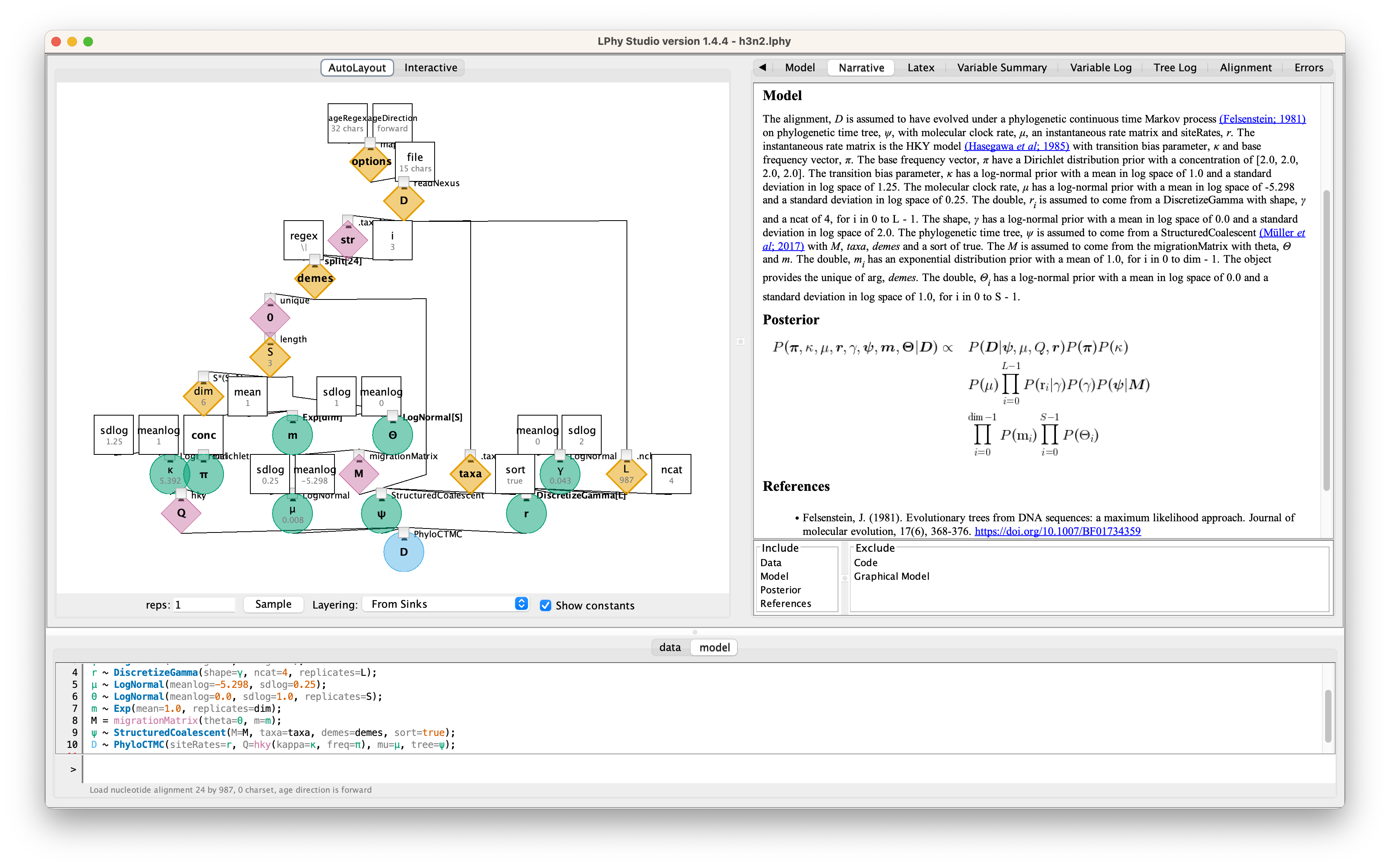
For the details, please read the auto-generated narrative from LPhyStudio.
Data block
The data { ... } block is necessary when we use LPhy Studio to prepare
instruction input files for inference software (e.g., BEAST 2,
RevBayes, etc.).
The purpose of this block is to tell LPhy which nodes of our graphical
model are to be treated as known constants (and not to be
sampled by the inference software) because they are observed
data.
Elsewhere, this procedure has been dubbed “clamping” (Höhna et al.,
2016).
In this block, we will either type strings representing values to be directly assigned to scalar variables, or use LPhy’s syntax to extract such values from LPhy objects, which might be read from file paths given by the user.
(Note that keyword data cannot be used to name variables because it
is reserved for defining scripting blocks as outlined above.)
In order to start specifying the data { ... } block, make sure you
type into the “data” tab of the command prompt, by clicking “data” at
the bottom of LPhy Studio’s window.
Tip dates
As the sequences were sampled through time, it’s necessary to specify their sampling dates,
which are included in the sequence names separated by |.
To extract and set the sampling dates, we utilize the regular expression
".*\|.*\|(\d*\.\d+|\d+\.\d*)\|.*$"
to extract the decimal numbers representing the dates and convert them into ages for further analysis.
How to set the age direction in LPhy is available in the tutorial Time-stamped data.
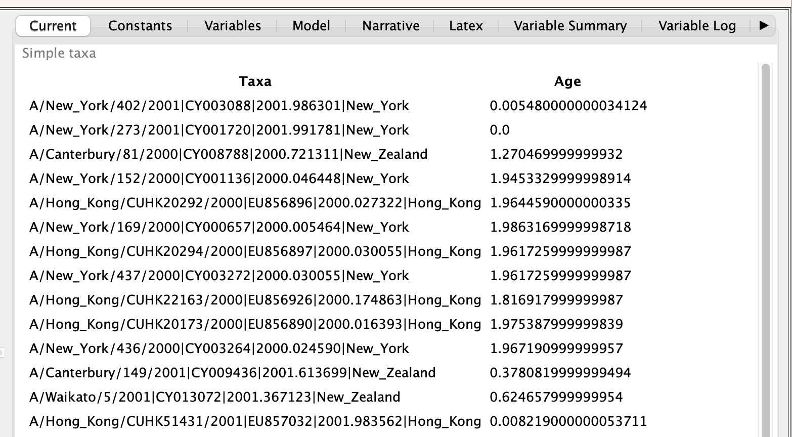
Tip locations
For this analyses we have additional information about
the sampling location of sequences taken from patients,
which are including Hong Kong, New York and New Zealand.
We can extract these sampling locations from taxa labels,
using split given the separator |, and taking the 4th element given i=3
where i is the index of split elements and starting from 0.
You can check them by clicking the graphical component demes (yellow orange diamond)
generated by the data section.
It is an array of locations required by the StructuredCoalescent in the model section later.
Model block
The model { ... } block is the main protagonist of our scripts.
This is where you will specify the many nodes and sampling
distributions that characterize a probabilistic model.
(Note that keyword model cannot be used to name variables because it
is reserved for defining scripting blocks as outlined above.)
In order to start specifying the model { ... } block, make sure you
type into the “model” tab of the command prompt, by clicking “model”
at the bottom of LPhy Studio’s window.
In this analysis, we will use three HKY models with estimated frequencies.
Additionally, we allow for rate heterogeneity among sites.
We do this by approximating the continuous rate distribution (for each site in the alignment)
with a discretized gamma probability distribution (mean = 1),
where the number of bins in the discretization ncat = 4 (normally between 4 and 6).
The shape parameter will be estimated in this analysis.
More details can be seen in the Bayesian Skyline Plots tutorial.
Next, we are going to set the priors for MASCOT. First, consider the effective population size parameter. Since we have only a few samples per location, meaning little information about the different effective population sizes, we will need an informative prior. In this case we will use a log normal prior with parameters M=0 and S=1. (These are respectively the mean and variance of the corresponding normal distribution in log space.)
The existing exponential distribution as a prior on the migration rate puts much weight on lower values while not prohibiting larger ones. For migration rates, a prior that prohibits too large values while not greatly distinguishing between very small and very very small values is generally a good choice. Be aware however that the exponential distribution is quite an informative prior: one should be careful that to choose a mean so that feasible rates are at least within the 95% HPD interval of the prior. (This can be determined by using R script)
A more in depth explanation of what backwards migration really are can be found in the Peter Beerli’s blog post.
Finally, set the prior for the clock rate. We have a good idea about the clock rate of Influenza A/H3N2 Hemagglutinin.
From previous work by other people, we know that the clock rate will be around 0.005 substitution per site per year.
To include that prior knowledger, we can set the prior on the clock rate to a log normal distribution.
If we set meanlog=-5.298 and sdlog=0.25, then we expect the clock rate to be with 95% certainty between 0.00306 and 0.00816.
Please note the dimension of effective population sizes should equal to
the number of locations (assuming it is x),
then the dimension of migration rates backwards in time should equal to
x*(x-1).
Producing BEAST XML using LPhyBEAST
BEAST 2 retrieves the data and model specifications from a XML file. One of our goals with LPhy is to make configuring Bayesian phylogenetic analysis as painless, clear and precise as possible. In order to achieve that, we will utilize an additional companion application called LPhyBEAST, which acts as a bridge between the LPhy script and the BEAST 2 xml. It is distributed as a BEAST 2 package, please follow the instruction to install it.
To run LPhyBEAST and produce a BEAST 2 xml, you need to use the terminal
and execute the script lphybeast.
The LPhyBEAST usage can help you get started.
In our h3n2.lphy script, the alignment file is assumed to be located
under the subfolder tutorials/data/.
To generate the XML, navigate to the tutorials folder where LPhy is installed,
and run the following command in your terminal.
After it completes, check the message in the end to find the location of the generated XML file.
For example, on a Mac, after replacing all “x” with the correct version number,
you can execute the following lphybeast command in the terminal to launch LPhyBEAST:
# go to the folder containing lphy script
cd /Applications/lphystudio-1.x.x/tutorials
# run lphybeast
'/Applications/BEAST 2.7.x/bin/lphybeast' -l 3000000 h3n2.lphy
If you are not familiar with inputting valid paths in the command line, here is our Tech Help that may help you.
For Windows users, please note that “C:\Program Files” is usually a protected directory.
However, you can copy the “examples” and “tutorials” folders with “data”
into your “Documents” folder and work in that location to avoid any permission issues.
Alternatively, run lphybeast.bat on a Windows terminal like this:
# go to the subfolder containing lphy script
cd "C:\Users\<YourUserName>\Documents\tutorials"
# run lphybeast
"C:\Program Files\BEAST2.7.x\bat\lphybeast.bat" -l 3000000 h3n2.lphy
Please note that the single or double quotation marks ensure that the whitespace in the path is treated as valid.
The -l option allows you to modify the MCMC chain length in the XML,
which is set to the default of 1 million.
Running BEAST
After LPhyBEAST generates a BEAST 2 .xml file (e.g., h3n2.xml), we can use BEAST 2 to load it and start the inferential MCMC analysis. BEAST 2 will write its outputs to disk into specified files in the XML, and also output the progress of the analysis and some summaries to the screen.
                        BEAST v2.7.5, 2002-2023
             Bayesian Evolutionary Analysis Sampling Trees
                       Designed and developed by
 Remco Bouckaert, Alexei J. Drummond, Andrew Rambaut & Marc A. Suchard

                   Centre for Computational Evolution
                         University of Auckland
                       r.bouckaert@auckland.ac.nz
                        alexei@cs.auckland.ac.nz

                   Institute of Evolutionary Biology
                        University of Edinburgh
                           a.rambaut@ed.ac.uk

                    David Geffen School of Medicine
                 University of California, Los Angeles
                           msuchard@ucla.edu

                      Downloads, Help & Resources:
                           http://beast2.org/

  Source code distributed under the GNU Lesser General Public License:
                   http://github.com/CompEvol/beast2

                           BEAST developers:
   Alex Alekseyenko, Trevor Bedford, Erik Bloomquist, Joseph Heled,
 Sebastian Hoehna, Denise Kuehnert, Philippe Lemey, Wai Lok Sibon Li,
Gerton Lunter, Sidney Markowitz, Vladimir Minin, Michael Defoin Platel,
          Oliver Pybus, Tim Vaughan, Chieh-Hsi Wu, Walter Xie

                               Thanks to:
          Roald Forsberg, Beth Shapiro and Korbinian Strimmer

Random number seed: 1690932416084

    ...

    ...
       28500000     -1946.4357     -1906.4363       -39.9993         0.3376         0.2286         0.2003         0.2333         3.7473         0.0042         0.4552         0.3231         0.4012         1.8612         0.0113         0.8998         0.2283         0.7402         1.5078         1.8011 50s/Msamples
       30000000     -1946.7403     -1901.9474       -44.7929         0.3505         0.2235         0.2021         0.2237         5.7619         0.0043         0.2648         3.4546         0.7509         0.4917         0.1204         0.8566         0.0782         4.7174         0.8943         0.5094 50s/Msamples

Operator                                                                  Tuning    #accept    #reject      Pr(m)  Pr(acc|m)
ScaleOperator(Theta.scale)                                               0.19597     233548     630013    0.02879    0.27045
ScaleOperator(gamma.scale)                                               0.16159     115908     283810    0.01334    0.28997
ScaleOperator(kappa.scale)                                               0.30351     106626     293099    0.01334    0.26675
ScaleOperator(m.scale)                                                   0.15631     387027    1014635    0.04677    0.27612
ScaleOperator(mu.scale)                                                  0.51995      99865     300853    0.01334    0.24922
beast.base.inference.operator.UpDownOperator(muUppsiDownOperator)        0.85804     319081    3382795    0.12343    0.08619 Try setting scaleFactor to about 0.926
beast.base.inference.operator.DeltaExchangeOperator(pi.deltaExchange)    0.07867     183781     680682    0.02879    0.21260
Exchange(psi.narrowExchange)                                                   -    1651694    1942594    0.11981    0.45953
ScaleOperator(psi.rootAgeScale)                                          0.53344      67693     333303    0.01334    0.16881
ScaleOperator(psi.scale)                                                 0.84705     270186    3325308    0.11981    0.07515 Try setting scaleFactor to about 0.92
SubtreeSlide(psi.subtreeSlide)                                           1.29737     399548    3193177    0.11981    0.11121
Uniform(psi.uniform)                                                           -    2215989    1378030    0.11981    0.61658
Exchange(psi.wideExchange)                                                     -      91717    3503880    0.11981    0.02551
WilsonBalding(psi.wilsonBalding)                                               -     159578    3435581    0.11981    0.04439

     Tuning: The value of the operator's tuning parameter, or '-' if the operator can't be optimized.
    #accept: The total number of times a proposal by this operator has been accepted.
    #reject: The total number of times a proposal by this operator has been rejected.
      Pr(m): The probability this operator is chosen in a step of the MCMC (i.e. the normalized weight).
  Pr(acc|m): The acceptance probability (#accept as a fraction of the total proposals for this operator).


Total calculation time: 1524.787 seconds
Done!
Analysing the BEAST output
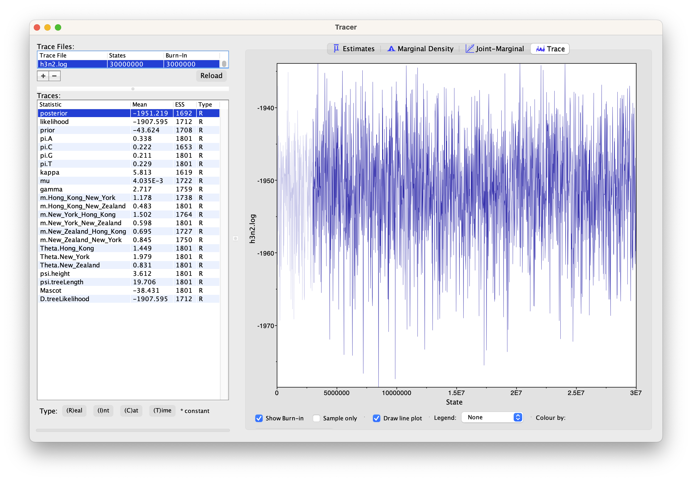
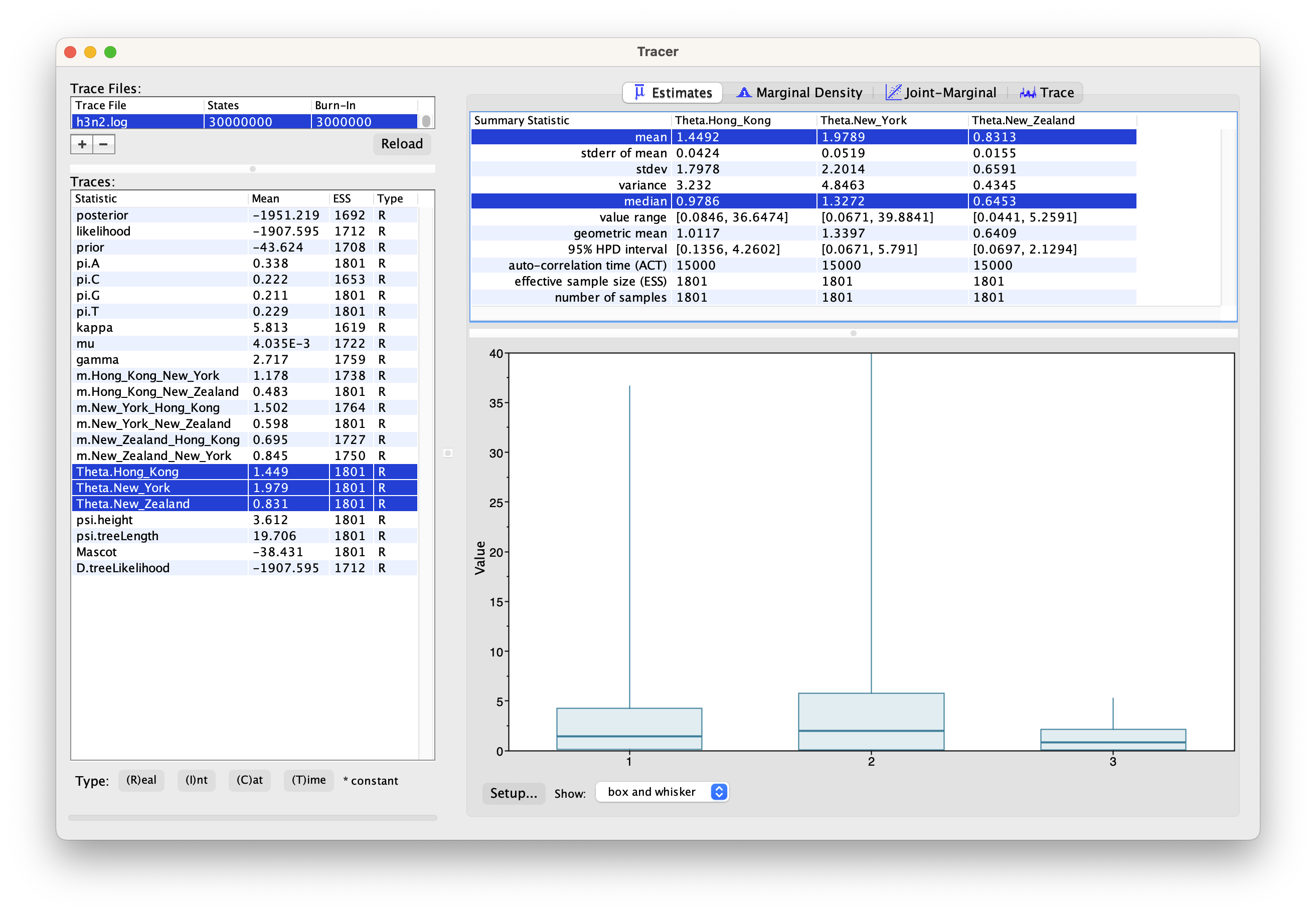
First, we can open the h3n2.log file in tracer to check if the MCMC has converged.
The ESS value should be above 200 for almost all values and especially for the posterior estimates.
We can have a look at the marginal posterior distributions for the effective population sizes. New York is inferred to have the largest effective population size before Hong Kong and New Zealand. This tells us that two lineages that are in New Zealand are expected to coalesce quicker than two lineages in Hong Kong or New York.
Tips: you can click the Setup... button to adjust the view range of X-axis.
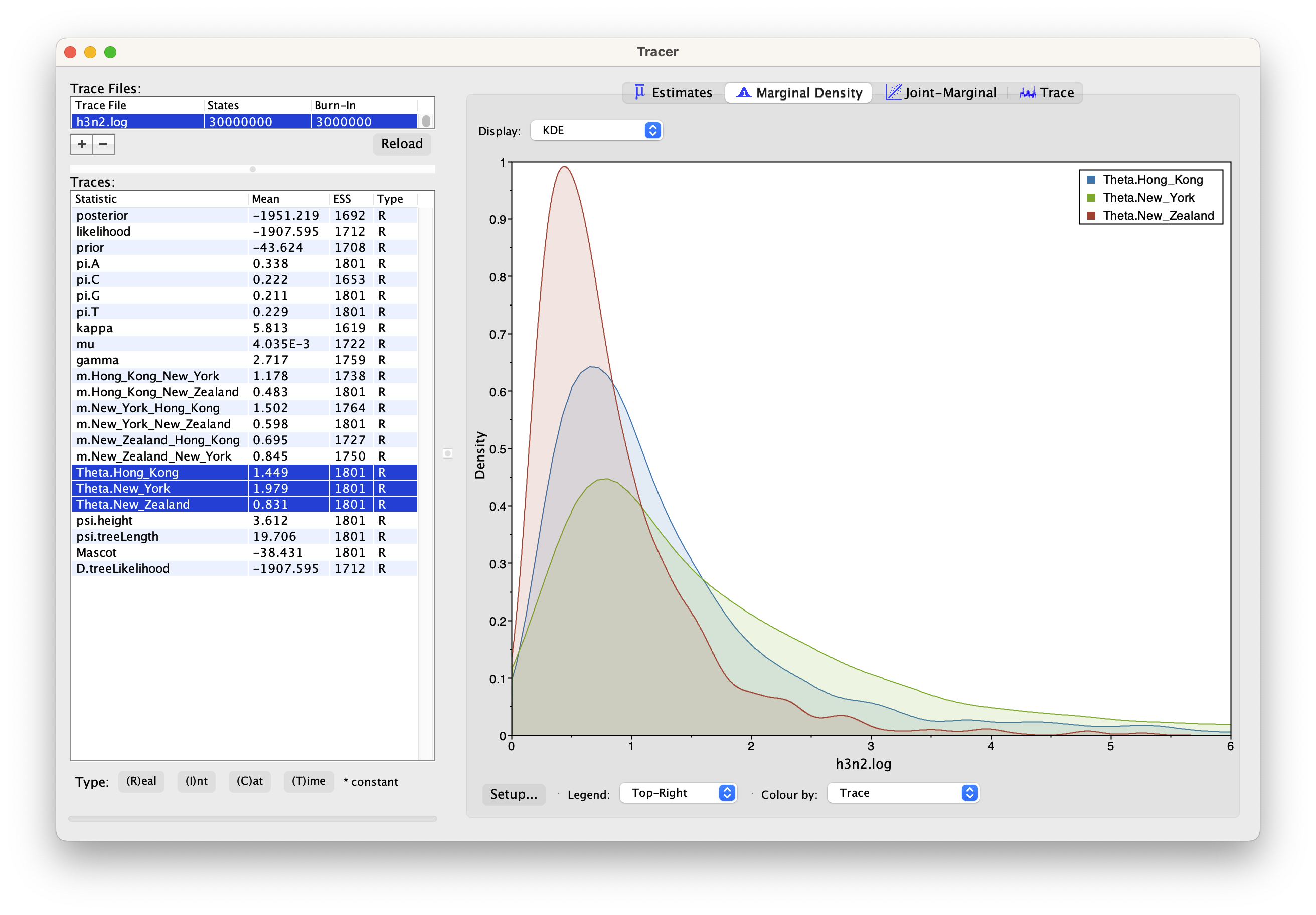
In this example, we have relatively little information about the effective population sizes of each location. This can lead to estimates that are greatly informed by the prior. Additionally, there can be great differences between median and mean estimates. The median estimates are generally more reliable since they are less influence by extreme values.
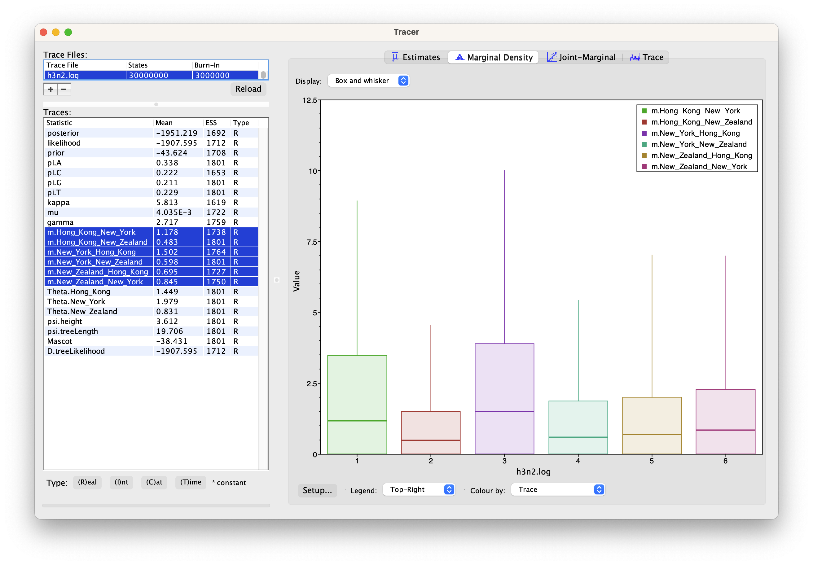
We can then look at the inferred migration rates.
The migration rates have the label b_m.*, meaning that they are backwards in time migration rates.
The highest rates are from New York to Hong Kong. Because they are backwards in time migration rates,
this means that lineages from New York are inferred to be likely from Hong Kong if we’re going backwards in time.
In the inferred phylogenies, we should therefore make the observation that lineages ancestral to samples from New York
are inferred to be from Hong Kong backwards.
Summarising the trees
To summarize the trees logged during MCMC, we will use the CCD methods implemented in the program TreeAnnotator to create the maximum a posteriori (MAP) tree. The implementation of the conditional clade distribution (CCD) offers different parameterizations, such as CCD1, which is based on clade split frequencies, and CCD0, which is based on clade frequencies. The MAP tree topology represents the tree topology with the highest posterior probability, averaged over all branch lengths and substitution parameter values.
You need to install CCD package to make the options available in TreeAnnotator.
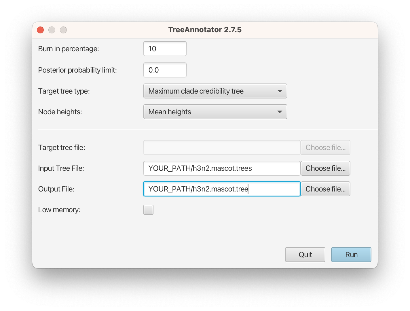
Please follow these steps after launching TreeAnnotator:
- Set 10% as the burn-in percentage;
- Select “MAP (CCD0)” as the “Target tree type”;
- For “Node heights”, choose “Common Ancestor heights”;
- Load the tree log file that BEAST 2 generated (it will end in “.trees” by default) as “Input Tree File”. For this tutorial, the tree log file is called h3n2.mascot.trees. If you select it from the file chooser, the parent path will automatically fill in and “YOUR_PATH” in the screen shot will be that parent path.
- Finally, for “Output File”, copy and paste the input file path but replace the h3n2.mascot.trees with h3n2.mascot.tree. This will create the file containing the resulting MAP tree.
The image below shows a screenshot of TreeAnnotator with the necessary settings to create the summary tree. “YOUR_PATH” will be replaced to the corresponding path.
The setup described above will take the set of trees in the tree log file and summarize it with a single MAP tree using the CCD0 method. Divergence times will reflect the average ages of each node summarised by the selected method, and these times will be annotated with their 95% highest posterior density (HPD) intervals. TreeAnnotator will also display the posterior clade credibility of each node in the MAP tree. More details on summarizing trees can be found in beast2.org/summarizing-posterior-trees/.
Note that TreeAnnotator only parses a tree log file into an output text file, but the visualization has to be done with other programs (see next section).
Visualizing the trees
In each logging step of the tree during the MCMC, MASCOT logs several different things. It logs the inferred probability of each node being in any possible location. In this example, these would be the inferred probabilities of being in Hong Kong, New York and New Zealand. Additonally, it logs the most likely location of each node.
After opening the MCC tree in FigTree, we can visualize several things.
To color branches, you can go to Appearance >> Colour by and select max.
This is the location that was inferred to be most often the most likely location of the node.
In addition, you can set the branch Width by max.prob, and increase the Line Weight, which will make the branch width more different regarding to its posterior support. Finally, tick Legend and select max in the drop list of Attribute.
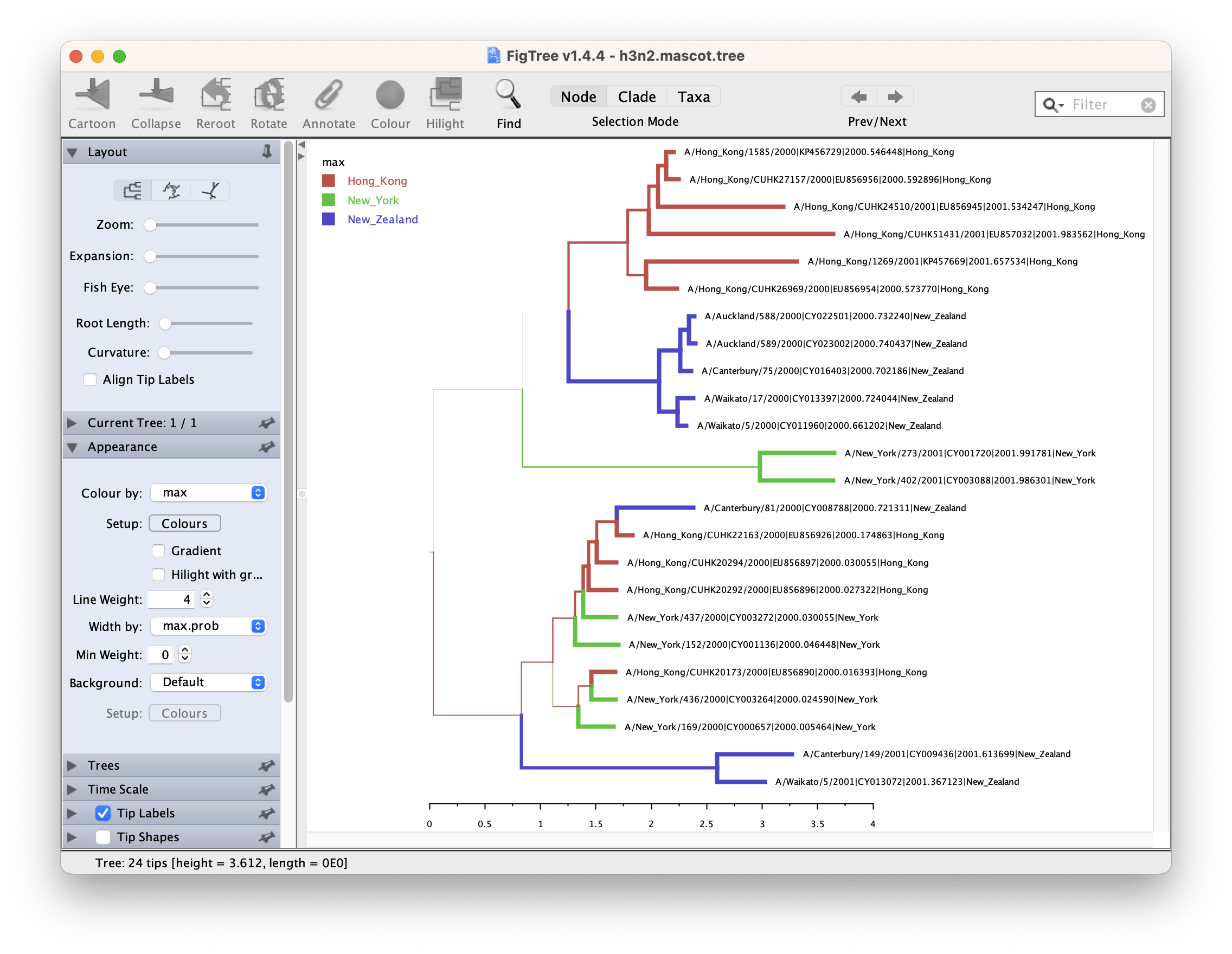
We can now determine if lineages ancestral to samples from New York are actually inferred to be from Hong Kong, or the probability of the root being in any of the locations.
To get the actual inferred probabilities of each node being in any of the 3 locations,
you can go to Node Labels >> Display an then choose Hong_Kong, New_York or New_Zealand.
These are the actual inferred probabilities of the nodes being in any location.
It should however be mentioned that the inference of nodes being in a particular location makes some simplifying assumptions, such as that there are no other locations (i.e. apart from the sampled locations) where lineages could have been.
Another important thing to know is that currently, we assume rates to be constant. This means that we assume that the population size of the different locations does not change over time. We also make the same assumption about the migration rates through time.
Questions
1. How to decide the dimensions of effective population sizes
   and migration rates respectively in an analysis?

2. How to interpret the differences among the effective population sizes?
   How to interpret the backwards migration rates?

3. How to determine the inferred locations of ancestral lineages?
   What assumptions are made on this result?
Errors that can occur (Work in progress)
One of the errors message that can occur regularly is the following: too many iterations, return negative infinity.
This occurs when the integration step size of the ODE’s
to compute the probability of observing a phylogenetic tree in MASCOT is becoming too small.
This generally occurs if at least one migration rate is really large or at least one effective population size is really small
(i.e. the coalescent rate is really high).
This causes integration steps to be extremely small,
which in turn would require a lot of time to compute the probability of a phylogenetic tree under MASCOT.
Instead of doing that, this state is rejected by assigning its log probability the value negative infinity.
This error can have different origins and a likely incomplete list is the following:
- The priors on migration rates put too much weight on really high rates. To fix this, reconsider your priors on the migration rates. Particularly, check if the prior on the migration rates make sense in comparison to the height of the tree. If, for example, the tree has a height of 1000 years, but the prior on the migration rate is exponential with mean 1, then the prior assumption is that between any two states, we expected approximately 1000 migration events.
- The prior on the effective population sizes is too low, meaning that the prior on the coalescent rates (1 over the effective population size) is too high. This can for example occur when the prior on the effective population size was chosen to be 1/X. To fix, reconsider your prior on the effective population size.
- There is substantial changes of the effective population sizes and/or migration rates over time that are not modeled. In that case, changes in the effective population sizes or migration rates have to be explained by population structure, which can again lead to some effective population sizes being very low and some migration rates being very high. In that case, there is unfortunately not much that can be done, since MASCOT is not an appropriate model for the dataset.
- There is strong subpopulation structure within the different subpopulations used. In that case, reconsider if the individual sub-populations used are reasonable.
Programs used in this tutorial
The following software will be used in this tutorial. We also offer a Tech Help page to assist you in case you encounter any unexpected issues with certain third-party software tools.
-
Java 17 or a later version is required by LPhy Studio.
-
LPhy Studio - This software will specify, visualize, and simulate data from models defined in LPhy scripts. At the time of writing, the current version is v1.7.x. It is available for download from LPhy releases.
-
LPhy BEAST - this BEAST 2 package will convert LPhy scripts into BEAST 2 XMLs. The installation guide and usage can be found from User Manual.
-
BEAST 2 - the bundle includes the BEAST 2 program, BEAUti, DensiTree, TreeAnnotator, and other utility programs. This tutorial is written for BEAST v2.7.x or higher version. It is available for download from http://www.beast2.org. Use
Package Managerto install the required BEAST 2 packages. -
BEAST labs package - this contains some generally useful stuff used by other BEAST 2 packages.
-
BEAST feast package - this is a small BEAST 2 package which contains additions to the core functionality.
-
BEAST CCD package - Implementation of the conditional clade distribution (CCD), such as, based on clade split frequencies (CCD1) and clade frequencies (CCD0). Furthermore, point estimators based on the CCDs are implemented, which allows TreeAnnotator to produce better summary trees than via MCC trees (which is restricted to the sample).
-
Tracer - this program is used to explore the output of BEAST (and other Bayesian MCMC programs). It graphically and quantitatively summarises the distributions of continuous parameters and provides diagnostic information. At the time of writing, the current version is v1.7.x. It is available for download from Tracer releases.
-
FigTree - this is an application for displaying and printing molecular phylogenies, in particular those obtained using BEAST. At the time of writing, the current version is v1.4.x. It is available for download from FigTree releases.
- MASCOT package - Marginal approximation of the structured coalescent.
- LPhyBeastExt package - The BEAST 2 package extended from the core project LPhyBeast, which includes Mascot LPhyBeast extension.
Data
Number of replicates, L is the number of characters of metadataalignment, D. The options are ageDirection="forward" and ageRegex=".*\|.*\|(\d*\.\d+|\d+\.\d*)\|.*$". Number of replicates, dim comes from the S*(S-1). The integer, S is the length of an object. The string, demes0 is assumed to come from the split with a str of "A/New_York/402/2001|CY003088|2001.986301|New_York", a regex of "\|" and an i of 3. The taxa is the list of taxa of metadataalignment, D.Model
The alignment, D is assumed to have evolved under a phylogenetic continuous time Markov process (Felsenstein; 1981) on phylogenetic time tree, ψ, with molecular clock rate, μ, an instantaneous rate matrix and siteRates, r. The instantaneous rate matrix is the HKY model (Hasegawa et al; 1985) with transition bias parameter, κ and base frequency vector, π. The base frequency vector, π have a Dirichlet distribution prior with a concentration of [2.0, 2.0, 2.0, 2.0]. The transition bias parameter, κ has a log-normal prior with a mean in log space of 1.0 and a standard deviation in log space of 1.25. The molecular clock rate, μ has a log-normal prior with a mean in log space of -5.298 and a standard deviation in log space of 0.25. The double, ri is assumed to come from a DiscretizeGamma with shape, γ and a ncat of 4, for i in 0 to L - 1. The shape, γ has a log-normal prior with a mean in log space of 0.0 and a standard deviation in log space of 2.0. The phylogenetic time tree, ψ is assumed to come from a StructuredCoalescent (Müller et al; 2017) with M, taxa, demes and a sort of true. The M is assumed to come from the migrationMatrix with theta, Θ and m. The double, mi has an exponential distribution prior with a mean of 1.0, for i in 0 to dim - 1. The object provides the unique of arg, demes. The double, Θi has a log-normal prior with a mean in log space of 0.0 and a standard deviation in log space of 1.0, for i in 0 to S - 1.Posterior
$$ \begin{split} P(\boldsymbol{\pi}, \kappa, \mu, \boldsymbol{r}, \gamma, \boldsymbol{\psi}, \boldsymbol{m}, \boldsymbol{\Theta} | \boldsymbol{D}) \propto &P(\boldsymbol{D} | \boldsymbol{\psi}, \mu, Q, \boldsymbol{r})P(\boldsymbol{\pi})P(\kappa)\\& P(\mu)\prod_{i=0}^{L - 1}P(\textrm{r}_i | \gamma)P(\gamma)P(\boldsymbol{\psi} | \boldsymbol{M})\\& \prod_{i=0}^{\textrm{dim} - 1}P(\textrm{m}_i)\prod_{i=0}^{S - 1}P(\Theta\textrm{}_i)\\& \end{split} $$XML and log files
- h3n2.xml
- h3n2.log
- h3n2.mascot.trees
- summarised tree h3n2.mascot.tree
Useful Links
If you interested in the derivations of the marginal approximation of the structured coalescent, you can find them from Müller, Rasmussen, & Stadler, 2017. This paper also explains the mathematical differences to other methods such as the theory underlying BASTA. To get a better idea of how the states of internal nodes are calculated, have a look in this paper Müller, Rasmussen, & Stadler, 2018.
- MASCOT source code: https://github.com/nicfel/Mascot
- LinguaPhylo: https://linguaphylo.github.io
- BEAST 2 website and documentation: http://www.beast2.org/
- Join the BEAST user discussion: http://groups.google.com/group/beast-users
References
- Felsenstein, J. (1981). Evolutionary trees from DNA sequences: a maximum likelihood approach. Journal of molecular evolution, 17(6), 368-376. https://doi.org/10.1007/BF01734359
- Hasegawa, M., Kishino, H. & Yano, T. Dating of the human-ape splitting by a molecular clock of mitochondrial DNA. J Mol Evol 22, 160–174 (1985) https://doi.org/10.1007/BF02101694
- Müller, N. F., Rasmussen, D., & Stadler, T. (2018). MASCOT: Parameter and state inference under the marginal structured coalescent approximation. Bioinformatics, bty406. https://doi.org/10.1093/bioinformatics/bty406
- Müller, N. F., Rasmussen, D. A., & Stadler, T. (2017). The Structured Coalescent and its Approximations. Molecular Biology and Evolution, msx186.
- Drummond, A. J., & Bouckaert, R. R. (2014). Bayesian evolutionary analysis with BEAST 2. Cambridge University Press.