Bayesian Skyline Plots
by LinguaPhylo core team
This tutorial is modified from Taming the BEAST tutorial Skyline plots.
If you haven’t installed LPhy Studio and LPhyBEAST yet, please refer to the User Manual for their installation. Additionally, this tutorial requires other third-party programs, which are listed below under the section Programs used in this tutorial.
Population dynamics influence the shape of the tree and consequently, the shape of the tree contains some information about past population dynamics. The so-called Skyline methods allow to extract this information from phylogenetic trees in a non-parametric manner. It is non-parametric since there is no underlying system of differential equations governing the inference of these dynamics.
In this tutorial we will look at a popular coalescent method, the Coalescent Bayesian Skyline plot (Drummond, Rambaut, Shapiro, & Pybus, 2005), to infer these dynamics from sequence data.
Background: Classic and Generalized Plots
(Drummond, Rambaut, Shapiro, & Pybus, 2005) explained these concepts in the figure below:
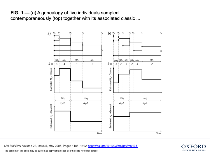
- A genealogy of five individuals sampled contemporaneously (top) together with its associated classic (middle) and generalized (bottom) skyline plots.
- A genealogy of five individuals sampled at three different times (top) along with its associated classic (middle) and generalized (bottom) skyline plots.
In the classic skyline plots, the changes in effective population size coincide with coalescent events,
resulting in a stepwise function with n − 2 change points and n − 1 population sizes,
where n is the number of sampled individuals.
In the generalized skyline plot, changes in effective population size coincide with some, but not necessarily all, coalescent events.
The resulting stepwise function has m − 1 change points (1 ≤ m ≤ n−1) and m effective population sizes.
The NEXUS alignment
The data is available in a file named hcv.nex. If you have installed LPhy Studio, you don’t need to download the data separately. It comes bundled with the studio and can be accessed in the “tutorials/data” subfolder within the installation directory of LPhy Studio.
The dataset consists of an alignment of 63 Hepatitis C sequences sampled in 1993 in Egypt (Ray, Arthur, Carella, Bukh, & Thomas, 2000). This dataset has been used previously to test the performance of skyline methods (Drummond, Rambaut, Shapiro, & Pybus, 2005, and Stadler, Kuhnert, Bonhoeffer, & Drummond, 2013).
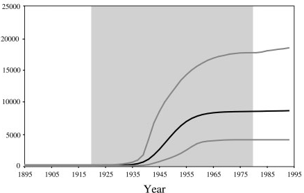
With an estimated 15-25%, Egypt has the highest Hepatits C prevalence in the world. In the mid 20th century, the prevalence of Hepatitis C increased drastically (see Figure 2 for estimates). We will try to infer this increase from sequence data.
Inputting the script into LPhy Studio
LPhy Studio implements a GUI for users to specify and visualize probabilistic graphical models, as well as for simulating data under those models. These tasks are executed according to an LPhy script the user types (or loads) on LPhy Studio’s interactive terminal. If you are not familiar with LPhy language, we recommend reading the language features before getting started.
You can input a script into LPhy Studio either by using the File menu
or by directly typing or pasting the script code into the console in LPhy Studio.
Please note if you are working in the console,
you do not need to add data and model keywords and curly brackets to define the code blocks.
We are supposed to add the lines without the data { } and model { } to the command line console
at the bottom of the window, where the data and model tabs in the GUI are used to specify
which block we are working on.
Below, we will build an LPhy script in two parts, the data and
the model blocks.
Code
data {D = readNexus(file="data/hcv.nexus");
L = D.nchar();
numGroups = 4;
taxa = D.taxa();
w = taxa.length()-1;
}
model {
π ~ Dirichlet(conc=[3.0, 3.0, 3.0, 3.0]);
rates ~ Dirichlet(conc=[1.0, 2.0, 1.0, 1.0, 2.0, 1.0]);
Q = gtr(rates=rates, freq=π);
γ ~ LogNormal(meanlog=0.0, sdlog=2.0);
r ~ DiscretizeGamma(shape=γ, ncat=4, replicates=L);
A ~ RandomComposition(k=numGroups, n=w);
θ1 ~ LogNormal(meanlog=9.0, sdlog=2.0);
Θ ~ ExpMarkovChain(firstValue=θ1, n=numGroups);
ψ ~ SkylineCoalescent(groupSizes=A, taxa=taxa, theta=Θ);
D ~ PhyloCTMC(Q=Q, mu=7.9E-4, siteRates=r, tree=ψ);
}
Graphical Model
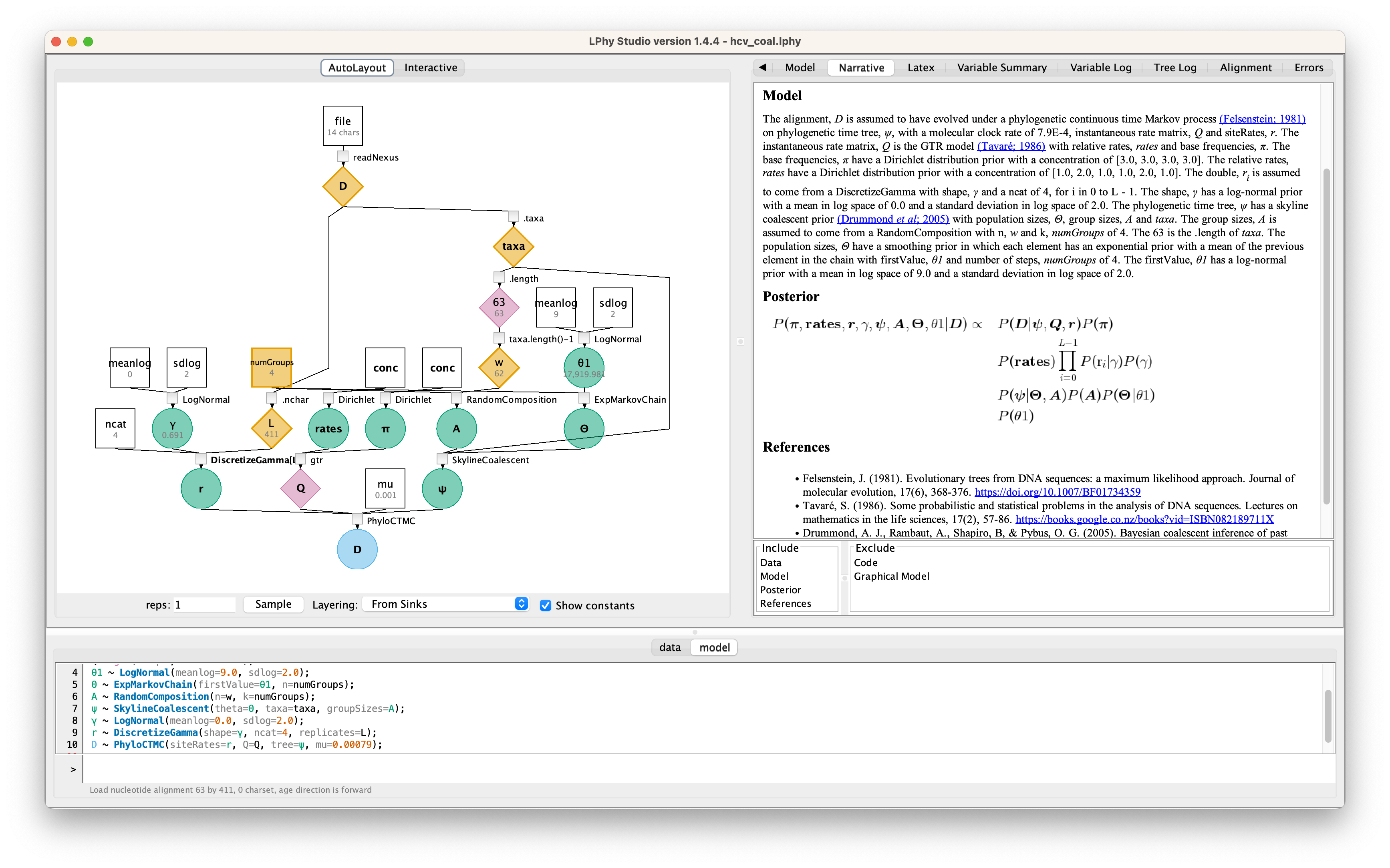
For the details, please read the auto-generated narrative from LPhyStudio.
Data block
The data { ... } block is necessary when we use LPhy Studio to prepare
instruction input files for inference software (e.g., BEAST 2,
RevBayes, etc.).
The purpose of this block is to tell LPhy which nodes of our graphical
model are to be treated as known constants (and not to be
sampled by the inference software) because they are observed
data.
Elsewhere, this procedure has been dubbed “clamping” (Höhna et al.,
2016).
In this block, we will either type strings representing values to be directly assigned to scalar variables, or use LPhy’s syntax to extract such values from LPhy objects, which might be read from file paths given by the user.
(Note that keyword data cannot be used to name variables because it
is reserved for defining scripting blocks as outlined above.)
In order to start specifying the data { ... } block, make sure you
type into the “data” tab of the command prompt, by clicking “data” at
the bottom of LPhy Studio’s window.
In the script, taxa and L respectively stores the taxa from the alignment D and the length of D.
numGroups = 4 sets the number of grouped intervals in the generalized Coalescent Bayesian Skyline plots,
and w defines n − 1 effective population sizes, which is the same number of times at which coalescent events occur.
Model block
The model { ... } block is the main protagonist of our scripts.
This is where you will specify the many nodes and sampling
distributions that characterize a probabilistic model.
(Note that keyword model cannot be used to name variables because it
is reserved for defining scripting blocks as outlined above.)
In order to start specifying the model { ... } block, make sure you
type into the “model” tab of the command prompt, by clicking “model”
at the bottom of LPhy Studio’s window.
In this analysis, we will use the GTR model, which is the most general reversible model and estimates transition probabilities between individual nucleotides separately. That means that the transition probabilities between e.g. A and T will be inferred separately to the ones between A and C, however transition probabilities from A to C will be the same as C to A etc. The nucleotide equilibrium state frequencies π are estimated here.
Additionally, we allow for rate heterogeneity among sites.
We do this by approximating the continuous rate distribution (for each site in the alignment)
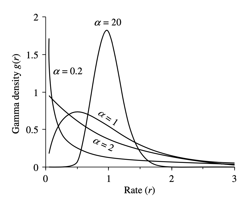
with a discretized gamma probability distribution (mean = 1),
where the number of bins in the discretization ncat = 4 (normally between 4 and 6).
The shape parameter will be estimated in this analysis.
As explained in (Yang, 2006), the shape parameter α is inversely related to the extent of rate variation at sites. If α > 1, the distribution is bell-shaped, meaning that most sites have intermediate rates around 1, while few sites have either very low or very high rates. In particular, when α → ∞, the distribution degenerates into the model of a single rate for all sites. If α ≤ 1, the distribution has a highly skewed L-shape, meaning that most sites have very low rates of substitution or are nearly ‘invariable’, but there are some substitution hotspots with high rates.
The sequences were all sampled in 1993 so we are dealing with a homochronous alignment and do not need to specify tip dates.
Because our sequences are contemporaneous (homochronous data), there is no information in our dataset to estimate the clock rate. We will use an estimate inferred in Pybus et al., 2001 to fix the clock rate. In this case all the samples were contemporaneous (sampled at the same time) and the clock rate is simply a scaling of the estimated tree branch lengths (in substitutions/site) into calendar time.
So, let’s set the clock rate $\mu$ to 0.00079 s/s/y
In addition, we define the priors for the following parameters:
- the vector of effective population sizes Θ;
- the relative rates of the GTR process rates;
- the base frequencies π;
- the shape of the discretized gamma distribution $\gamma$.
Here we setup a Markov chain of effective population sizes using ExpMarkovChain,
and apply a LogNormal distribution to the first value of the chain.
Please note that the first value Θ1 is measured from the tips according to
(Drummond, Rambaut, Shapiro, & Pybus, 2005).
The vector of group sizes A are positive integers randomly sampled by the function RandomComposition
where the vector’s dimension equals to a constant numGroups,
and they should sum to the number of coalescent events w.
Questions
-
What are
numGroupsandwaccording to the Figure 1? And how to compute the number of coalescent events given the number of taxa? -
How to change the above LPhy scripts to use the classic Skyline coalescent?
Tips: by default all group sizes in SkylineCoalescent function are 1 which is equivalent to the classic skyline coalescent.
Producing BEAST XML using LPhyBEAST
BEAST 2 retrieves the data and model specifications from a XML file. One of our goals with LPhy is to make configuring Bayesian phylogenetic analysis as painless, clear and precise as possible. In order to achieve that, we will utilize an additional companion application called LPhyBEAST, which acts as a bridge between the LPhy script and the BEAST 2 xml. It is distributed as a BEAST 2 package, please follow the instruction to install it.
To run LPhyBEAST and produce a BEAST 2 xml, you need to use the terminal
and execute the script lphybeast.
The LPhyBEAST usage can help you get started.
In our hcv_coal.lphy script, the alignment file is assumed to be located
under the subfolder tutorials/data/.
To generate the XML, navigate to the tutorials folder where LPhy is installed,
and run the following command in your terminal.
After it completes, check the message in the end to find the location of the generated XML file.
For example, on a Mac, after replacing all “x” with the correct version number,
you can execute the following lphybeast command in the terminal to launch LPhyBEAST:
# go to the folder containing lphy script
cd /Applications/lphystudio-1.x.x/tutorials
# run lphybeast
'/Applications/BEAST 2.7.x/bin/lphybeast' -l 40000000 hcv_coal.lphy
If you are not familiar with inputting valid paths in the command line, here is our Tech Help that may help you.
For Windows users, please note that “C:\Program Files” is usually a protected directory.
However, you can copy the “examples” and “tutorials” folders with “data”
into your “Documents” folder and work in that location to avoid any permission issues.
Alternatively, run lphybeast.bat on a Windows terminal like this:
# go to the subfolder containing lphy script
cd "C:\Users\<YourUserName>\Documents\tutorials"
# run lphybeast
"C:\Program Files\BEAST2.7.x\bat\lphybeast.bat" -l 40000000 hcv_coal.lphy
Please note that the single or double quotation marks ensure that the whitespace in the path is treated as valid.
The -l option allows you to modify the MCMC chain length in the XML,
which is set to the default of 1 million.
Running BEAST
After LPhyBEAST generates a BEAST 2 .xml file (e.g., hcv_coal.xml), we can use BEAST 2 to load it and start the inferential MCMC analysis. BEAST 2 will write its outputs to disk into specified files in the XML, and also output the progress of the analysis and some summaries to the screen.
                        BEAST v2.7.8, 2002-2025
             Bayesian Evolutionary Analysis Sampling Trees
                       Designed and developed by
 Remco Bouckaert, Alexei J. Drummond, Andrew Rambaut & Marc A. Suchard

                   Centre for Computational Evolution
                         University of Auckland
                       r.bouckaert@auckland.ac.nz
                        alexei@cs.auckland.ac.nz

                   Institute of Evolutionary Biology
                        University of Edinburgh
                           a.rambaut@ed.ac.uk

                    David Geffen School of Medicine
                 University of California, Los Angeles
                           msuchard@ucla.edu

                      Downloads, Help & Resources:
                           http://beast2.org/

  Source code distributed under the GNU Lesser General Public License:
                   http://github.com/CompEvol/beast2

                           BEAST developers:
   Alex Alekseyenko, Trevor Bedford, Erik Bloomquist, Joseph Heled,
 Sebastian Hoehna, Denise Kuehnert, Philippe Lemey, Wai Lok Sibon Li,
Gerton Lunter, Sidney Markowitz, Vladimir Minin, Michael Defoin Platel,
          Oliver Pybus, Tim Vaughan, Chieh-Hsi Wu, Walter Xie

                               Thanks to:
          Roald Forsberg, Beth Shapiro and Korbinian Strimmer

Random number seed: 1690761608289

    ...

    ...
       38000000     -6682.0050     -6201.7299      -480.2750         0.1921         0.3048         0.2408         0.2621         0.0571         0.3585         0.0448         0.0230         0.4713         0.0451         0.3280             11              2             37             12      9413.8662      4976.3181       227.2886       431.5181 1m23s/Msamples
       40000000     -6625.8487     -6178.0316      -447.8170         0.1904         0.3316         0.2480         0.2298         0.0579         0.3502         0.0629         0.0258         0.4559         0.0471         0.4004              9             47              4              2     11386.5587       188.1198       317.8618        48.4388 1m23s/Msamples

Operator                                                                                    Tuning    #accept    #reject      Pr(m)  Pr(acc|m)
beast.base.inference.operator.kernel.BactrianDeltaExchangeOperator(A.deltaExchange)        2.49956     263985     683360    0.02368    0.27866
kernel.BactrianScaleOperator(Theta.scale)                                                  0.66248     355150     801911    0.02896    0.30694
kernel.BactrianScaleOperator(gamma.scale)                                                  0.16866     129408     309379    0.01097    0.29492
beast.base.inference.operator.kernel.BactrianDeltaExchangeOperator(pi.deltaExchange)       0.04474     271745     674029    0.02368    0.28733
EpochFlexOperator(psi.BICEPSEpochAll)                                                      0.25113     280127     432406    0.01783    0.39314
EpochFlexOperator(psi.BICEPSEpochTop)                                                      0.25252     171950     266858    0.01097    0.39186
TreeStretchOperator(psi.BICEPSTreeFlex)                                                    0.09311    3149381    4743648    0.19725    0.39901
Exchange(psi.narrowExchange)                                                                     -    3173854    4718140    0.19725    0.40216
kernel.BactrianScaleOperator(psi.rootAgeScale)                                             0.26334      25933     412407    0.01097    0.05916 Try setting scale factor to about 0.132
kernel.BactrianSubtreeSlide(psi.subtreeSlide)                                             15.42851    1268695    6615536    0.19725    0.16092
kernel.BactrianNodeOperator(psi.uniform)                                                   1.94902    2462884    5429179    0.19725    0.31207
Exchange(psi.wideExchange)                                                                       -       8636     993577    0.02505    0.00862
WilsonBalding(psi.wilsonBalding)                                                                 -      14557     986842    0.02505    0.01454
beast.base.inference.operator.kernel.BactrianDeltaExchangeOperator(rates.deltaExchange)    0.19638       8125    1348299    0.03385    0.00599 Try setting delta to about 0.098

     Tuning: The value of the operator's tuning parameter, or '-' if the operator can't be optimized.
    #accept: The total number of times a proposal by this operator has been accepted.
    #reject: The total number of times a proposal by this operator has been rejected.
      Pr(m): The probability this operator is chosen in a step of the MCMC (i.e. the normalized weight).
  Pr(acc|m): The acceptance probability (#accept as a fraction of the total proposals for this operator).


Total calculation time: 3358.018 seconds
Done!
Analysing the BEAST output
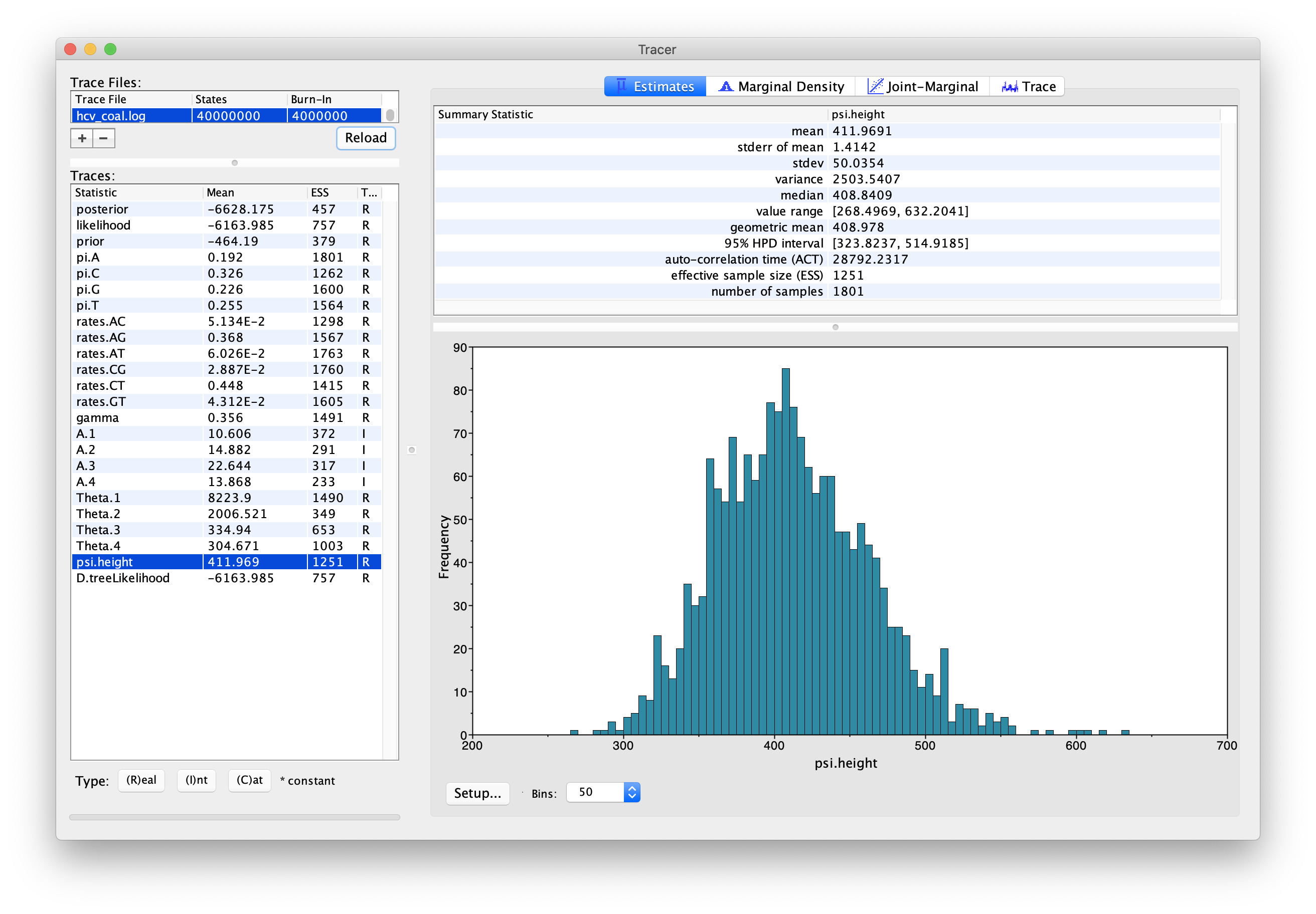
Run the program called Tracer to analyze the output of BEAST. When the
main window has opened, choose Import Trace File... from the File menu
and select the file that BEAST has created called hcv_coal.log.
You should now see a window like in 5.
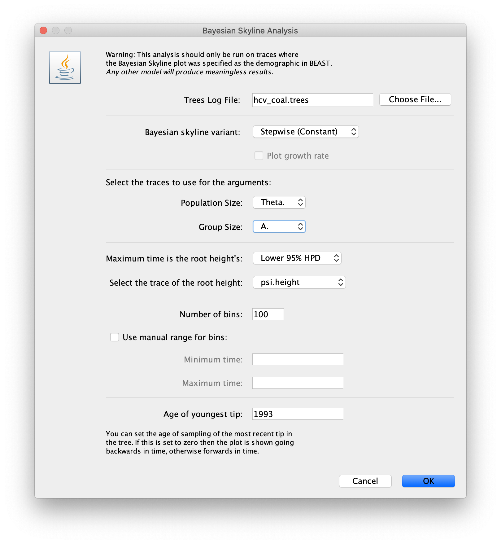
For the reconstruction of the population dynamics, we need two files, the hcv_coal.log file and the hcv_coal.trees file.
The log file contains the information about the group sizes and population sizes of each segment,
while the trees file is needed for the times of the coalescent events.
Navigate to Analysis > Bayesian Skyline Reconstruction.
From there open the tree log file. To get the correct dates in the analysis we should specify the Age of the youngest tip.
In our case it is 1993, the year where all the samples were taken.
If the sequences were sampled at different times (heterochronous data),
the age of the youngest tip is the time when the most recent sample was collected.
Press OK to reconstruct the past population dynamics.
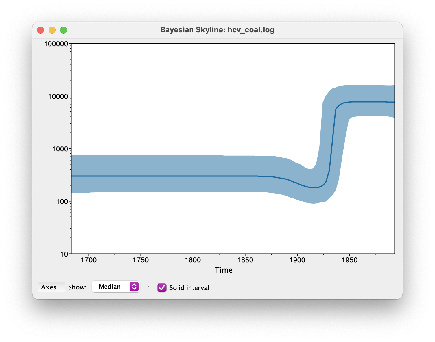
The output will have the years on the x-axis and the effective population size on the y-axis. By default, the y-axis is on a log-scale. If everything worked as it is supposed to work you will see a sharp increase in the effective population size in the mid 20th century, similar to what is seen below.
Note that the reconstruction will only work if the *.log and *.trees files contain the same number of states and both files were logged at the same frequency.
There are two ways to save the analysis, it can either be saved as a PDF file for displaying purposes or as a tab delimited file.
Navigate to File > Export Data Table. Enter the filename as hcv_coal.tsv and save the file.
The exported file will have five rows, the time, the mean, median, lower and upper boundary of the 95% HPD interval of the estimates,
which you can use to plot the data with other software (R, Matlab, etc).
The parameterization and choosing the dimension
Please read the section of “The Coalescent Bayesian Skyline parameterization” and “Choosing the Dimension” from Taming the BEAST tutorial Skyline plots.
Questions
-
How to choose the dimension for the Bayesian skyline analysis? How does the number of dimensions of effective population sizes affect the result?
-
What are the alternative models to deal with this dimension problem?
-
What does the Bayesian skyline plot in this analysis tell you?
Some considerations for using skyline plots
In the coalescent, the time is modeled to go backwards, from present to past.
The coalescent skylines assume that the population is well-mixed. That is, they assume that there is no significant population structure and that the sequences are a random sample from the population. However, if there is population structure, for instance sequences were sampled from two different villages and there is much more contact within than between villages, then the results will be biased (Heller, Chikhi, & Siegismund, 2013). Instead a structured model should then be used to account for these biases.
Programs used in this tutorial
The following software will be used in this tutorial. We also offer a Tech Help page to assist you in case you encounter any unexpected issues with certain third-party software tools.
-
Java 17 or a later version is required by LPhy Studio.
-
LPhy Studio - This software will specify, visualize, and simulate data from models defined in LPhy scripts. At the time of writing, the current version is v1.7.x. It is available for download from LPhy releases.
-
LPhy BEAST - this BEAST 2 package will convert LPhy scripts into BEAST 2 XMLs. The installation guide and usage can be found from User Manual.
-
BEAST 2 - the bundle includes the BEAST 2 program, BEAUti, DensiTree, TreeAnnotator, and other utility programs. This tutorial is written for BEAST v2.7.x or higher version. It is available for download from http://www.beast2.org. Use
Package Managerto install the required BEAST 2 packages. -
BEAST labs package - this contains some generally useful stuff used by other BEAST 2 packages.
-
BEAST feast package - this is a small BEAST 2 package which contains additions to the core functionality.
-
BEAST CCD package - Implementation of the conditional clade distribution (CCD), such as, based on clade split frequencies (CCD1) and clade frequencies (CCD0). Furthermore, point estimators based on the CCDs are implemented, which allows TreeAnnotator to produce better summary trees than via MCC trees (which is restricted to the sample).
-
Tracer - this program is used to explore the output of BEAST (and other Bayesian MCMC programs). It graphically and quantitatively summarises the distributions of continuous parameters and provides diagnostic information. At the time of writing, the current version is v1.7.x. It is available for download from Tracer releases.
-
FigTree - this is an application for displaying and printing molecular phylogenies, in particular those obtained using BEAST. At the time of writing, the current version is v1.4.x. It is available for download from FigTree releases.
-
BEAST SSM (standard substitution models) package - this BEAST 2 package contains the following standard time-reversible substitution models: JC, F81, K80, HKY, TrNf, TrN, TPM1, TPM1f, TPM2, TPM2f, TPM3, TPM3f, TIM1, TIM1f, TIM2, TIM2f, TIM3 , TIM3f, TVMf, TVM, SYM, GTR.
Data
The number of replicates, L is the number of characters of alignment, D. The alignment, D is read from the Nexus file with a file name of "data/hcv.nexus". numGroups = 4 The n, w is calculated by taxa.length()-1. The taxa is the list of taxa of alignment, D.Model
The alignment, D is assumed to have evolved under a phylogenetic continuous time Markov process (Felsenstein; 1981) on phylogenetic time tree, ψ, with a molecular clock rate of 7.9E-4, instantaneous rate matrix, Q and siteRates, r. The instantaneous rate matrix, Q is the general time-reversible rate matrix (Rodriguez et al; 1990) with relative rates, rates and base frequencies, π. The base frequencies, π have a Dirichlet distribution prior with a concentration of [3.0, 3.0, 3.0, 3.0]. The relative rates, rates have a Dirichlet distribution prior with a concentration of [1.0, 2.0, 1.0, 1.0, 2.0, 1.0]. The double, ri is assumed to come from a DiscretizeGamma with shape, γ and a ncat of 4, for i in 0 to L - 1. The shape, γ has a log-normal prior with a mean in log space of 0.0 and a standard deviation in log space of 2.0. The phylogenetic time tree, ψ has a skyline coalescent prior (Drummond et al; 2005) with population sizes, Θ, group sizes, A and taxa. The group sizes, A is assumed to come from a RandomComposition with n, w and k, numGroups of 4. The taxa.length() is the .length of taxa. The population sizes, Θ have a smoothing prior in which each element has an exponential prior with a mean of the previous element in the chain with firstValue, θ1 and number of steps, numGroups of 4. The firstValue, θ1 has a log-normal prior with a mean in log space of 9.0 and a standard deviation in log space of 2.0.Posterior
$$ \begin{split} P(\boldsymbol{\pi}, \boldsymbol{\textbf{rates}}, \boldsymbol{r}, \gamma, \boldsymbol{\psi}, \boldsymbol{A}, \boldsymbol{\Theta}, \theta1 | \boldsymbol{D}) \propto &P(\boldsymbol{D} | \boldsymbol{\psi}, \boldsymbol{Q}, \boldsymbol{r})P(\boldsymbol{\pi})\\& P(\boldsymbol{\textbf{rates}})\prod_{i=0}^{L - 1}P(\textrm{r}_i | \gamma)P(\gamma)\\& P(\boldsymbol{\psi} | \boldsymbol{\Theta}, \boldsymbol{A})P(\boldsymbol{A})P(\boldsymbol{\Theta} | \theta1)\\& P(\theta1)\end{split} $$XML and log files
- hcv_coal.xml
- hcv_coal.log
- hcv_coal.trees
- summarised tree hcv_coal.tree
Useful Links
- LinguaPhylo: https://linguaphylo.github.io
- BEAST 2 website and documentation: http://www.beast2.org/
- Join the BEAST user discussion: http://groups.google.com/group/beast-users
References
- Drummond, A. J., Rambaut, A., Shapiro, B., & Pybus, O. G. (2005). Bayesian coalescent inference of past population dynamics from molecular sequences. Molecular Biology and Evolution, 22(5), 1185–1192. https://doi.org/10.1093/molbev/msi103
- Bouckaert, R., Heled, J., Kühnert, D., Vaughan, T., Wu, C.-H., Xie, D., … Drummond, A. J. (2014). BEAST 2: a software platform for Bayesian evolutionary analysis. PLoS Computational Biology, 10(4), e1003537. https://doi.org/10.1371/journal.pcbi.1003537
- Bouckaert, R., Vaughan, T. G., Barido-Sottani, J., Duchêne, S., Fourment, M., Gavryushkina, A., … Drummond, A. J. (2019). BEAST 2.5: An advanced software platform for Bayesian evolutionary analysis. PLOS Computational Biology, 15(4).
- Ray, S. Ê. C., Arthur, R. Ê. R., Carella, A., Bukh, J., & Thomas, D. Ê. L. (2000). Genetic Epidemiology of Hepatitis C Virus throughout Egypt. The Journal of Infectious Diseases, 182(3), 698–707. https://doi.org/10.1086/315786
- Pybus, O. G., Drummond, A. J., Nakano, T., Robertson, B. H., & Rambaut, A. (2003). The Epidemiology and Iatrogenic Transmission of Hepatitis C Virus in Egypt: A Bayesian Coalescent Approach. Molecular Biology and Evolution, 20(3), 381–387. https://doi.org/10.1093/molbev/msg043
- Pybus, O. G., Charleston, M. A., Gupta, S., Rambaut, A., Holmes, E. C., Harvey, P. H., … Felsenstein, J. (2001). The epidemic behavior of the hepatitis C virus. Science (New York, N.Y.), 292(5525), 2323–2325. https://doi.org/10.1126/science.1058321
- Rosenberg, N. A., & Nordborg, M. (2002). Genealogical trees, coalescent theory and the analysis of genetic polymorphisms. Nature Reviews Genetics, 3(5).
- Pybus, O. G., Rambaut, A., & Harvey, P. H. (2000). An Integrated Framework for the Inference of Viral Population History From Reconstructed Genealogies. Genetics, 155(3).
- Heled, J., & Drummond, A. J. (2008). Bayesian inference of population size history from multiple loci. BMC Evolutionary Biology, 8(1), 289. https://doi.org/10.1186/1471-2148-8-289
- Minin, V. N., Bloomquist, E. W., & Suchard, M. A. (2008). Smooth skyride through a rough skyline: Bayesian coalescent-based inference of population dynamics. Molecular Biology and Evolution, 25(7), 1459–1471. https://doi.org/10.1093/molbev/msn090
- Heller, R., Chikhi, L., & Siegismund, H. R. (2013). The confounding effect of population structure on Bayesian skyline plot inferences of demographic history. PloS One, 8(5), e62992. https://doi.org/10.1371/journal.pone.0062992
- Drummond, A. J., & Bouckaert, R. R. (2014). Bayesian evolutionary analysis with BEAST 2. Cambridge University Press.