Time-stamped data
by Fábio K. Mendes, Walter Xie, Eva Li and Alexei J. Drummond
This tutorial is modified from Taming the BEAST material. You can find the source tutorial, data and author information here.
Requirements
The programs used in this tutorial are listed below. In case you have not done it yet, please follow the installation instructions here before moving on.
Background
In this tutorial, we will study the phylodynamics of the Respiratory syncytial virus subgroup A (RSVA). RSVA infects the human lower respiratory tract, causing symptoms that are often indistinguishable from the common cold. By age 3, nearly all children will be infected, and a small percentage (<3%) will develop a more serious inflammation of the bronchioles requiring hospitalisation.
Goals
The goal of our phylodynamic analysis is to estimate:
- the rate of molecular evolution (of RSVA’s G gene);
- the date of the most recent common ancestor (MRCA) of all viral samples (i.e., the tree’s root), interpreted as the first infection event with respect to the samples at hand;
- the phylogenetic relationships among viral samples.
Data
Our data is comprised of 129 molecular sequences coding for RSVA’s G protein (Zlateva et al., 2004; Zlateva et al., 2005), a glycoprotein that allows the virus to attach itself to the host cells’ membranes, starting the infection. Importantly, our data is time stamped (also referred to as heterochronous or serial data) because it was collected at multiple time points, from 1956–2002.
Below we further detail how we will treat our molecular data in our analyses.
The NEXUS alignment
The data is available in a file named RSV2.nex. If you have installed LPhy Studio, you don’t need to download the data separately. It comes bundled with the studio and can be accessed in the “tutorials/data” subfolder within the installation directory of LPhy Studio.
Multiple partitions
Our molecular alignment corresponds to a 629-bp coding sequence of RSVA’s G protein. We are going to partition our alignment into three compartments corresponding to the first, second and third codon positions.
Tip dates
In phylodynamic and macroevolutionary analyses, quite often our samples (viral sequences from infected individuals in the former case and from different species in the latter, for example) were collected only at the present moment. In such cases we assign our samples an age of 0.0 to represent the present – this is our default.
As mentioned above, however, our sequences have been sampled at
various dates going back to the 1950s.
We can see the date of each of our samples (sequences) in the NEXUS
file, after the last lower-case s.
This date can be read as years since 1900.
Whenever tip dates are heterochronous and used as data, they can be read in natural forward time (here, we refer to them simply as “dates”) or backward time (in which case we call them “ages”).
Whether we treat the tip times as dates or ages internally in the code, however, depends on how the models we want to use are parameterized. The same goes for how we output the internal node times when we estimate them during phylogenetic inference. Regardless, the times are first converted into scalar values from 0.0 to some value > 0.0 (in days, years, millions of years, etc.).
LPhy’s behavior is to treat tip times always as ages.
Non-identifiability of rate and time
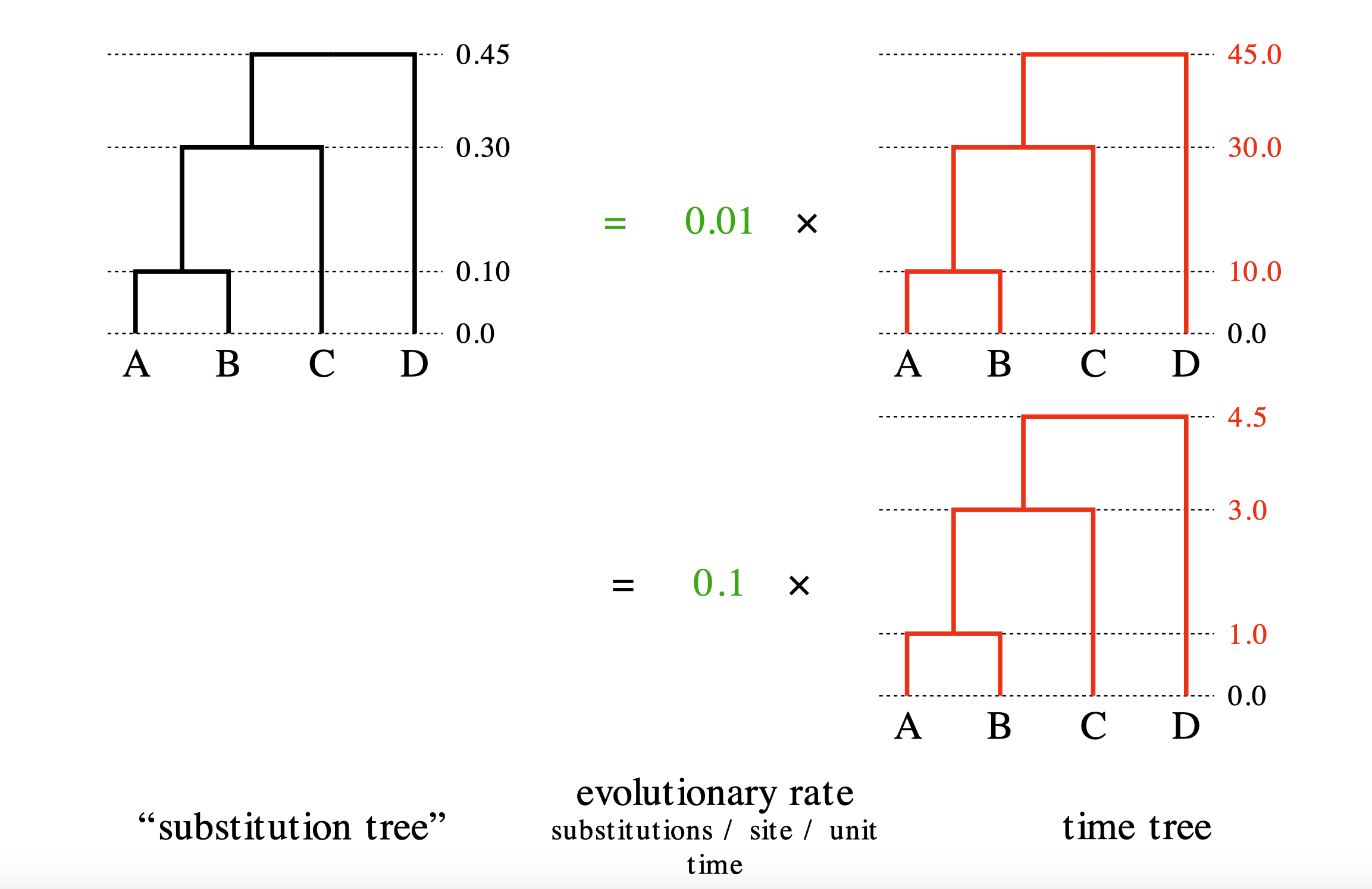
The strict molecular clock parameterization must satisfies genetic distance = rate × time.
We can compute genetic distance from an alignment using an evolutionary model such as HKY.
But we cannot determine whether the observed genetic distance is due to a fast rate over a short time
or a slow rate over a long time.
This problem is called the non-identifiability of rate and time.
To estimate mutation rates, you need additional information about time,
such as fossil ages or virus sample collection dates.
The detail is available in Prof. Alexei Drummond’s lecture slides.
Inputting the script into LPhy Studio
LPhy Studio implements a GUI for users to specify and visualize probabilistic graphical models, as well as for simulating data under those models. These tasks are executed according to an LPhy script the user types (or loads) on LPhy Studio’s interactive terminal. If you are not familiar with LPhy language, we recommend reading the language features before getting started.
You can input a script into LPhy Studio either by using the File menu
or by directly typing or pasting the script code into the console in LPhy Studio.
Please note if you are working in the console,
you do not need to add data and model keywords and curly brackets to define the code blocks.
We are supposed to add the lines without the data { } and model { } to the command line console
at the bottom of the window, where the data and model tabs in the GUI are used to specify
which block we are working on.
Below, we will build an LPhy script in two parts, the data and
the model blocks.
Data block
The data { ... } block is necessary when we use LPhy Studio to prepare
instruction input files for inference software (e.g., BEAST 2,
RevBayes, etc.).
The purpose of this block is to tell LPhy which nodes of our graphical
model are to be treated as known constants (and not to be
sampled by the inference software) because they are observed
data.
Elsewhere, this procedure has been dubbed “clamping” (Höhna et al.,
2016).
In this block, we will either type strings representing values to be directly assigned to scalar variables, or use LPhy’s syntax to extract such values from LPhy objects, which might be read from file paths given by the user.
(Note that keyword data cannot be used to name variables because it
is reserved for defining scripting blocks as outlined above.)
In order to start specifying the data { ... } block, make sure you
type into the “data” tab of the command prompt, by clicking “data” at
the bottom of LPhy Studio’s window.
options = {ageDirection="forward", ageRegex="s(\d+)$"};
D = readNexus(file="data/RSV2.nex", options=options);
codon = D.charset(["3-629\3", "1-629\3", "2-629\3"]);
L = codon.nchar();
n = length(codon);
taxa = D.taxa();
}
Our data here consist of molecular alignments and the sample dates.
We start by parsing the latter with regular expression "s(\d+)" when
defining some options in options={}.
This tells LPhy how to extract the sample times from the NEXUS file,
and then we specify that we want to read those times as dates (i.e.,
forward in time).
After all, our sample times are given to us in natural time.
In order to check if you have set the sample times correctly, click
the graphical component taxa and check the column “Age”.
The most recent sequences (i.e., from 2002 and that end with s102)
should have an age of 0.0, while all other tips should be > 0.0.
This is because, as mentioned above, LPhy always treats sample
times as ages.
The alignment D is imported from a Nexus file “RSV2.nex”.
The argument file="data/RSV2.nex" is used to look for this file under the relative path “data”,
with its parent directory being the current working directory.
However, this could lead to the issue
if the working directory is not the parent directory of “data”,
especially when using the LPhy Studio console.
To avoid potential issues with relative paths,
a simple solution is to use the absolute path in the argument file="...".
Then we must parse the molecular alignments by initializing the variable D.
Note that our open reading frame (ORF) starts at position 3.
This must be reflected in the arguments we pass to the charset() function to define the codon positions:
- first (
"3-629\3"), - second (
"1-629\3"), and - third (
"2-629\3").
The charset() function returns three alignments as a vector called codon.
Finally, we use the last three lines to set the number of loci L,
the number of taxa n, and the taxa themselves, taxa.
Note that n=length(codon); is equivalent to n=3; because
length() here is extracting the number of partitions in codon.
If you want to double-check everything you have typed, click the “Model” tab in the upper right panel.
Model block
The model { ... } block is the main protagonist of our scripts.
This is where you will specify the many nodes and sampling
distributions that characterize a probabilistic model.
(Note that keyword model cannot be used to name variables because it
is reserved for defining scripting blocks as outlined above.)
In order to start specifying the model { ... } block, make sure you
type into the “model” tab of the command prompt, by clicking “model”
at the bottom of LPhy Studio’s window.
We will specify sampling distributions for the following parameters, in this order:
π, the equilibrium nucleotide frequencies (with 4 dimensions, one for each nucleotide);κ, twice the transition:transversion bias assuming equal nucleotide frequencies (with 3 dimensions, one for each partition);r, the relative rates (with 3 dimensions, one for each partition);μ, the global (mean) molecular clock rate;Θ, the effective population size;ψ, the time-scaled phylogenetic tree, where the time unit is years.
π ~ Dirichlet(replicates=n, conc=[2.0, 2.0, 2.0, 2.0]);
κ ~ LogNormal(sdlog=0.5, meanlog=1.0, replicates=n);
r ~ WeightedDirichlet(conc=rep(element=1.0, times=n), weights=L);
μ ~ LogNormal(meanlog=-5.0, sdlog=1.25);
Θ ~ LogNormal(meanlog=3.0, sdlog=2.0);
ψ ~ Coalescent(taxa=taxa, theta=Θ);
codon ~ PhyloCTMC(L=L, Q=hky(kappa=κ, freq=π, meanRate=r), mu=μ, tree=ψ);
}
The parameter π represents the nucleotide equilibrium frequencies.
κ (kappa) specifies the transition/transversion rate ratio.
Both are defined as 3-dimensional vectors using the optional argument replicates=n, where n=3 in this case.
The parameter r defines the relative substitution rates
for each of the three codon partitions.
LPhy makes use of vectorization, so when WeightedDirichlet receives
a vector input (such as L being 3-dimensional),
it automatically constructs three separate relative rate vectors, one for each partition.
This same behavior applies to PhyloCTMC, which also handles vectorised inputs internally.
One final remark is that we use rep(element=1.0, times=n) (where n
evaluates to 3) to create three concentration vectors (one vector per
partition) for the WeightedDirichlet sampling distribution.
You can click the graphical components to view their simulated values. Again, if you want to double-check everything you have typed, click the “Model” tab in the upper right panel.
The whole script
Let us look at the whole thing:
data {options = {ageDirection="forward", ageRegex="s(\d+)$"};
D = readNexus(file="data/RSV2.nex", options=options);
codon = D.charset(["3-629\3", "1-629\3", "2-629\3"]);
L = codon.nchar();
n = length(codon);
taxa = D.taxa();
}
model {
π ~ Dirichlet(replicates=n, conc=[2.0, 2.0, 2.0, 2.0]);
κ ~ LogNormal(sdlog=0.5, meanlog=1.0, replicates=n);
r ~ WeightedDirichlet(conc=rep(element=1.0, times=n), weights=L);
μ ~ LogNormal(meanlog=-5.0, sdlog=1.25);
Θ ~ LogNormal(meanlog=3.0, sdlog=2.0);
ψ ~ Coalescent(taxa=taxa, theta=Θ);
codon ~ PhyloCTMC(L=L, Q=hky(kappa=κ, freq=π, meanRate=r), mu=μ, tree=ψ);
}
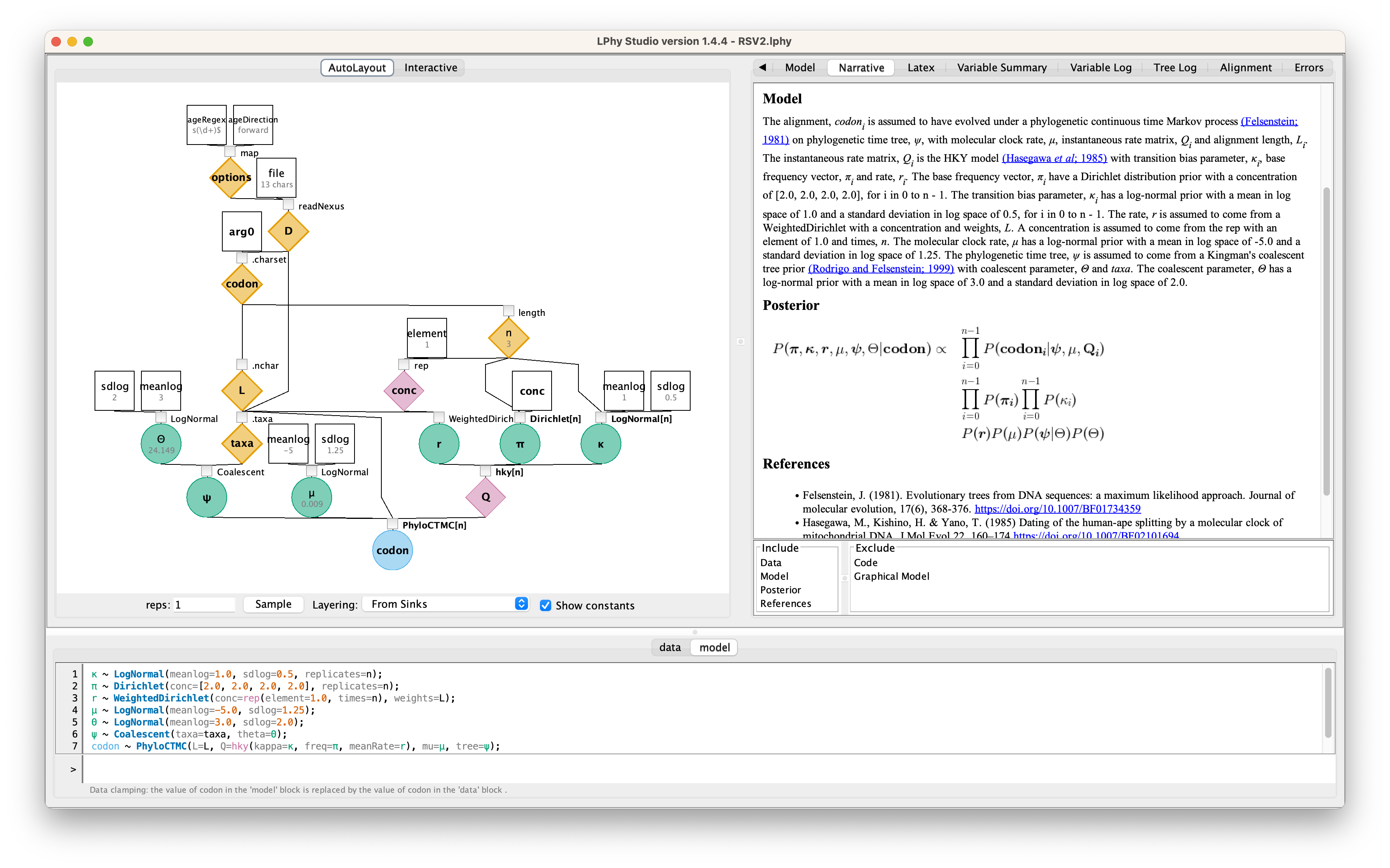
If the script contains no errors, you will be able to see the specified graphical model. Simulated data, such as the alignment and the tree, can be seen in the right-hand panel.
As alternatives to typing or copying-and-pasting the script above,
you can find it in HTML format here, or you can load
the script with “File” > “Tutorials Scripts” and select RSV2.lphy.
Phylogenetic inference with BEAST 2
Once we have read in our data and defined our model, we can move to the task of carrying out statistical inference. We shall try to estimate our parameters of interest, and for the purposes of this tutorial we will do that using the BEAST 2 program.
Producing a BEAST 2 .xml using LPhyBEAST
BEAST 2 retrieves the data and model specifications from a XML file. One of our goals with LPhy is to make configuring Bayesian phylogenetic analysis as painless, clear and precise as possible. In order to achieve that, we will utilize an additional companion application called LPhyBEAST, which acts as a bridge between the LPhy script and the BEAST 2 xml. It is distributed as a BEAST 2 package, please follow the instruction to install it.
To run LPhyBEAST and produce a BEAST 2 xml, you need to use the terminal
and execute the script lphybeast.
The LPhyBEAST usage can help you get started.
In our RSV2.lphy script, the alignment file is assumed to be located
under the subfolder tutorials/data/.
To generate the XML, navigate to the tutorials folder where LPhy is installed,
and run the following command in your terminal.
After it completes, check the message in the end to find the location of the generated XML file.
For example, on a Mac, after replacing all “x” with the correct version number,
you can execute the following lphybeast command in the terminal to launch LPhyBEAST:
# go to the folder containing lphy script
cd /Applications/lphystudio-1.x.x/tutorials
# run lphybeast
'/Applications/BEAST 2.7.x/bin/lphybeast' RSV2.lphy
If you are not familiar with inputting valid paths in the command line, here is our Tech Help that may help you.
For Windows users, please note that “C:\Program Files” is usually a protected directory.
However, you can copy the “examples” and “tutorials” folders with “data”
into your “Documents” folder and work in that location to avoid any permission issues.
Alternatively, run lphybeast.bat on a Windows terminal like this:
# go to the subfolder containing lphy script
cd "C:\Users\<YourUserName>\Documents\tutorials"
# run lphybeast
"C:\Program Files\BEAST2.7.x\bat\lphybeast.bat" RSV2.lphy
Please note that the single or double quotation marks ensure that the whitespace in the path is treated as valid.
Running BEAST 2
After LPhyBEAST generates a BEAST 2 .xml file (e.g., RSV2.xml), we can use BEAST 2 to load it and start the inferential MCMC analysis. BEAST 2 will write its outputs to disk into specified files in the XML, and also output the progress of the analysis and some summaries to the screen.
                        BEAST v2.7.8, 2002-2025
             Bayesian Evolutionary Analysis Sampling Trees
                       Designed and developed by
 Remco Bouckaert, Alexei J. Drummond, Andrew Rambaut & Marc A. Suchard

                   Centre for Computational Evolution
                         University of Auckland
                       r.bouckaert@auckland.ac.nz
                        alexei@cs.auckland.ac.nz

                   Institute of Evolutionary Biology
                        University of Edinburgh
                           a.rambaut@ed.ac.uk

                    David Geffen School of Medicine
                 University of California, Los Angeles
                           msuchard@ucla.edu

                      Downloads, Help & Resources:
                           http://beast2.org/

  Source code distributed under the GNU Lesser General Public License:
                   http://github.com/CompEvol/beast2

                           BEAST developers:
   Alex Alekseyenko, Trevor Bedford, Erik Bloomquist, Joseph Heled,
 Sebastian Hoehna, Denise Kuehnert, Philippe Lemey, Wai Lok Sibon Li,
Gerton Lunter, Sidney Markowitz, Vladimir Minin, Michael Defoin Platel,
          Oliver Pybus, Tim Vaughan, Chieh-Hsi Wu, Walter Xie

                               Thanks to:
          Roald Forsberg, Beth Shapiro and Korbinian Strimmer

Running file RSV2.xml
File: RSV2.xml seed: 2160030974204605245 threads: 1
    ...

    ...
         950000     -6093.6543     -5490.2432      -603.4110         0.4758         0.2259         0.0963         0.2018         0.2731         0.4117         0.1111         0.2038         0.3281         0.4085         0.0910         0.1722         8.1613         7.1496        11.6311         0.5955         1.0316         1.3709         0.0021        34.0876 55s/Msamples
        1000000     -6079.8549     -5484.0842      -595.7707         0.4530         0.2677         0.1107         0.1684         0.2896         0.4210         0.0976         0.1916         0.2989         0.3977         0.0739         0.2293         5.4948        10.4505        10.2371         0.6823         0.9759         1.3402         0.0024        37.4179 55s/Msamples

Operator                                                                                   Tuning    #accept    #reject      Pr(m)  Pr(acc|m)
kernel.BactrianScaleOperator(Theta.scale)                                                 0.21787       1449       4472    0.00586    0.24472
kernel.BactrianScaleOperator(kappa.scale)                                                 0.34910       3621       8889    0.01265    0.28945
kernel.BactrianScaleOperator(mu.scale)                                                    0.11193        918       4892    0.00586    0.15800
beast.base.inference.operator.kernel.BactrianUpDownOperator(muUppsiDownOperator)          0.11188        705     175870    0.17596    0.00399 Try setting scale factor to about 0.056
beast.base.inference.operator.kernel.BactrianDeltaExchangeOperator(pi_0.deltaExchange)    0.08504       2193      10184    0.01265    0.17718
beast.base.inference.operator.kernel.BactrianDeltaExchangeOperator(pi_1.deltaExchange)    0.06443       3476       9297    0.01265    0.27214
beast.base.inference.operator.kernel.BactrianDeltaExchangeOperator(pi_2.deltaExchange)    0.06726       2513      10167    0.01265    0.19819
EpochFlexOperator(psi.BICEPSEpochAll)                                                     0.07907       1002       8489    0.00952    0.10557
EpochFlexOperator(psi.BICEPSEpochTop)                                                     0.07882        609       5258    0.00586    0.10380
TreeStretchOperator(psi.BICEPSTreeFlex)                                                   0.02965      27125     147635    0.17501    0.15521
Exchange(psi.narrowExchange)                                                                    -      44841     130153    0.17501    0.25624
kernel.BactrianScaleOperator(psi.rootAgeScale)                                            0.33243         19       5817    0.00586    0.00326 Try setting scale factor to about 0.166
kernel.BactrianSubtreeSlide(psi.subtreeSlide)                                          1180.33719        190     175046    0.17501    0.00108 Try decreasing size to about 590.169
kernel.BactrianNodeOperator(psi.uniform)                                                  2.27178      60697     114054    0.17501    0.34733
Exchange(psi.wideExchange)                                                                      -         53      15505    0.01547    0.00341
WilsonBalding(psi.wilsonBalding)                                                                -        116      15178    0.01547    0.00758
beast.base.inference.operator.kernel.BactrianDeltaExchangeOperator(r.deltaExchange)       0.20272       2699       6869    0.00952    0.28209

     Tuning: The value of the operator's tuning parameter, or '-' if the operator can't be optimized.
    #accept: The total number of times a proposal by this operator has been accepted.
    #reject: The total number of times a proposal by this operator has been rejected.
      Pr(m): The probability this operator is chosen in a step of the MCMC (i.e. the normalized weight).
  Pr(acc|m): The acceptance probability (#accept as a fraction of the total proposals for this operator).


Total calculation time: 58.151 seconds
End likelihood: -6079.854960424774
Analysing BEAST 2’s output
We start by opening the Tracer program, and dropping the RSV2.log
file onto Tracer’s window.
Alternatively you can load the trace (.log) file by clicking “File” > “Import
Trace File…”.
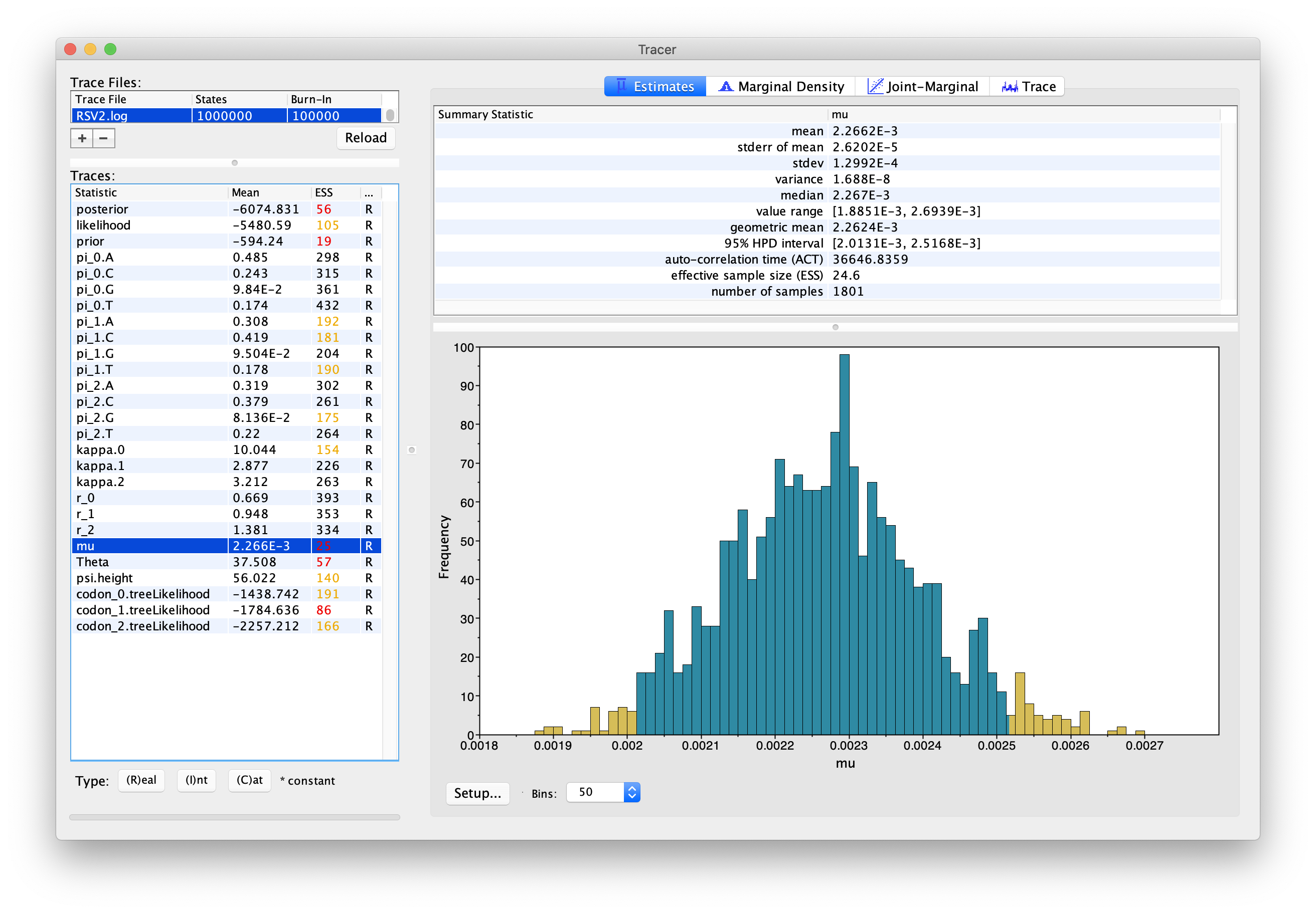
Tracer will display several summary statistics computed from the trace file in the left-hand and top-right panels. Other summaries will be displayed graphically. It is all pretty self-evident, just click around to familiarize yourself with the program.
The first thing you will notice from this first run is that the effective sample sizes (ESSs) for many of the logged quantities are small (ESSs less than 100 will be highlighted in red by Tracer). This is not good. A low ESS means that the trace contains a lot of correlated samples and thus may not represent the posterior distribution well. In the bottom-right panel you will see a histogram that looks a bit rough. This is expected when ESSs are low.
If you click the “Trace” tab in the upper-right corner, you will see the raw trace, that is, the sampled values against the step in the MCMC chain (Fig. 4).
The trace shows the value of a given statistic for each sampled step of the MCMC chain. It will help you see if the chain is mixing well and to what extent the samples are correlated. Here you can see how the samples are correlated.
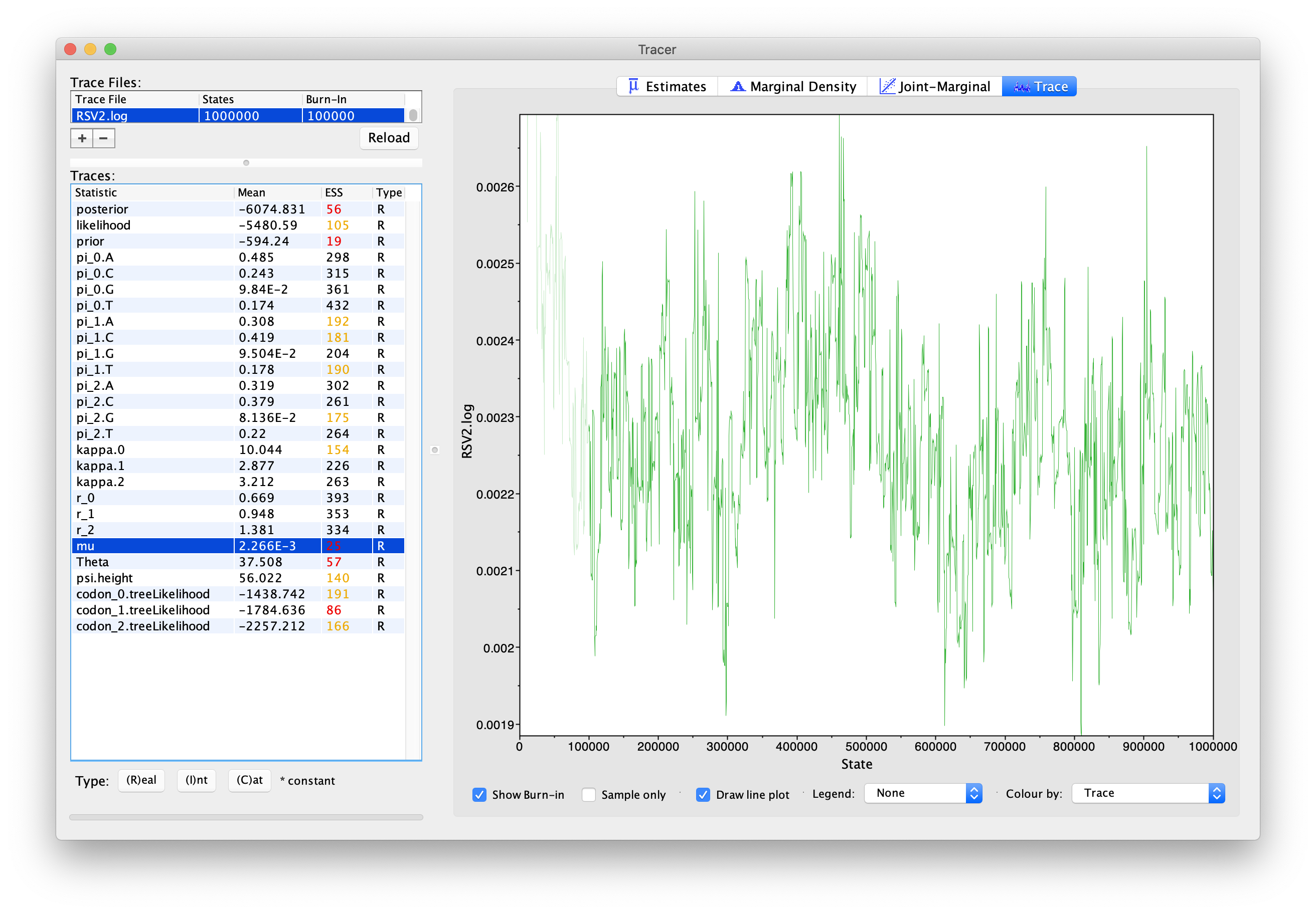
In LPhyBEAST, the default MCMC chain length is 1,000,000. After we remove the burn-in (set to 10%), there will be 1,800 samples in the trace (we ran the MCMC for steps sampling every 500). Note how adjacent samples often tend to have similar values – not great.
The ESS for the mean molecular clock rate (μ) is about 25 so we
are only getting 1 independent sample every 72 samples
(to a total of ~1800/25 “effective” samples).
With such a short run, it may also be the case that the default
burn-in of 10% of the chain length is inadequate.
Not excluding enough of the start of the chain as burn-in will render
estimates of ESS unreliable.
Let us try to fix this low ESS issue by running the MCMC chain for longer. We will set the chain length to 20,000,000, but still log the same number of samples (2,000). You can now run LPhyBEAST again create a new .xml file:
$BEAST_DIR/bin/lphybeast -l 20000000 -o RSV2long.xml RSV2.lphy
Two extra arguments:
-lchanges the MCMC chain length (default to 1 million) in the XML;-oreplaces the output file name (default to use the same file steam as the lphy input file).
Now run BEAST 2 with the new XML again.
It may take about half an hour to complete using modern computers.
If you do not want to wait, you can download the completed log and tree files
by running the longer MCMC chain.
Load the new log file into Tracer after it is finished (you can leave the old one loaded for comparison). Click on the “Trace” tab and look at the raw trace plot.
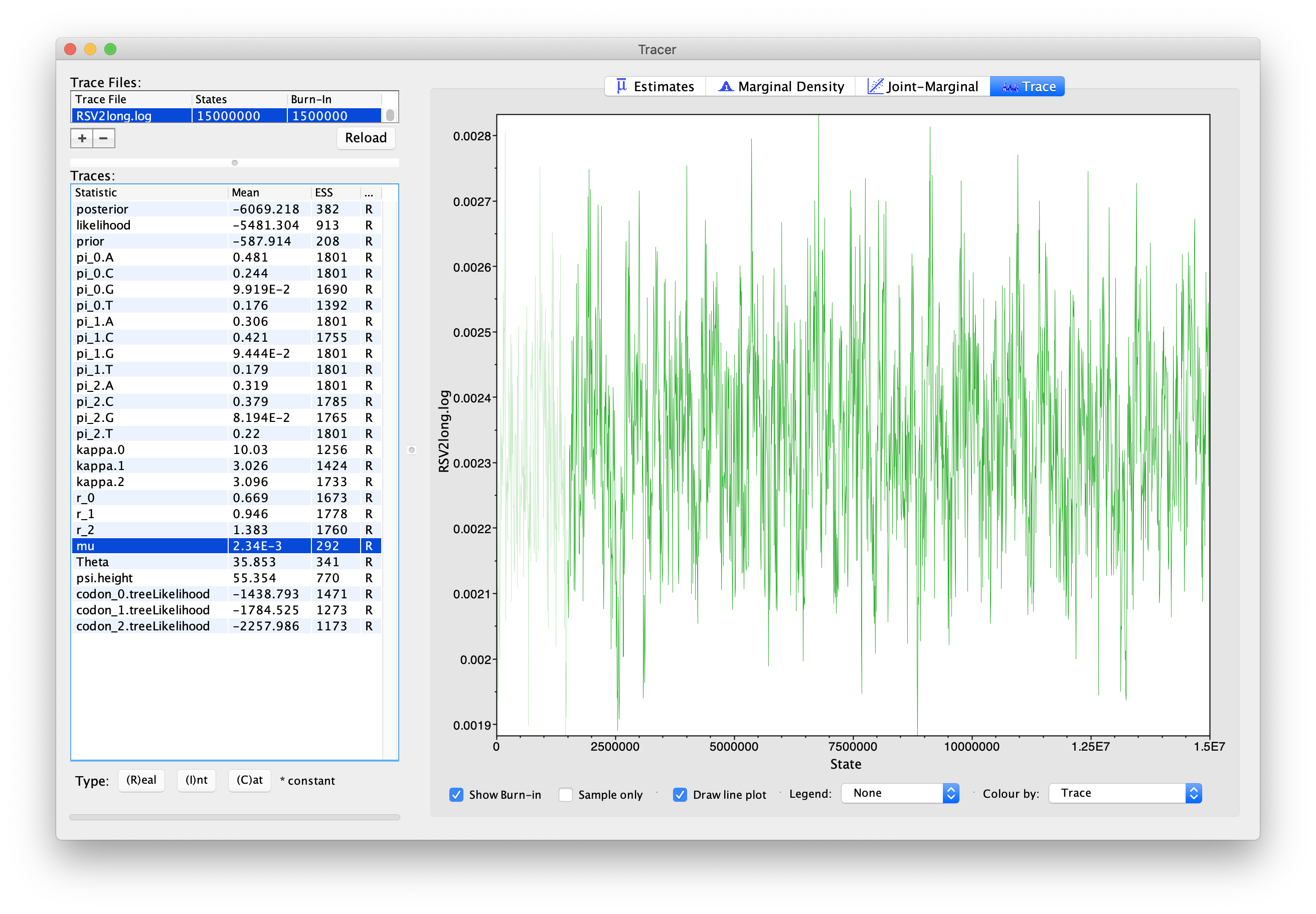
With this much longer MCMC chain, we still have 1,800 samples after removing the first 10% as burn-in, but our ESSs are all > 200. A large ESS does not mean there is no auto-correlation between samples overall, but instead that we have at least 200 effectively independent samples. More effective samples means we are approximating the posterior better than before, when ESSs were less than 100.
(You should keep an eye for weird trends in the trace plot suggesting that the MCMC chain has not yet converged, or is struggling to converge, like different value “plateaus” attracting the chain for a large number of steps.)
Empirically, the topology of posterior trees typically converges more slowly than other parameters because trees are multi-dimensional objects. To address this, we introduce a simple method to compute the Tree ESS using TreeStat2.
Now that we are satisfied with the length of the MCMC chain and its
mixing, we can move on to one of the parameters of interest: the
global clock rate, μ.
This is the average molecular clock rate across all sites in the
alignment.
First, select “mu” in the left-hand panel, and click the “Marginal Density” tab in the upper-right corner to see the posterior density plot for this parameter. You should see a plot similar to this:
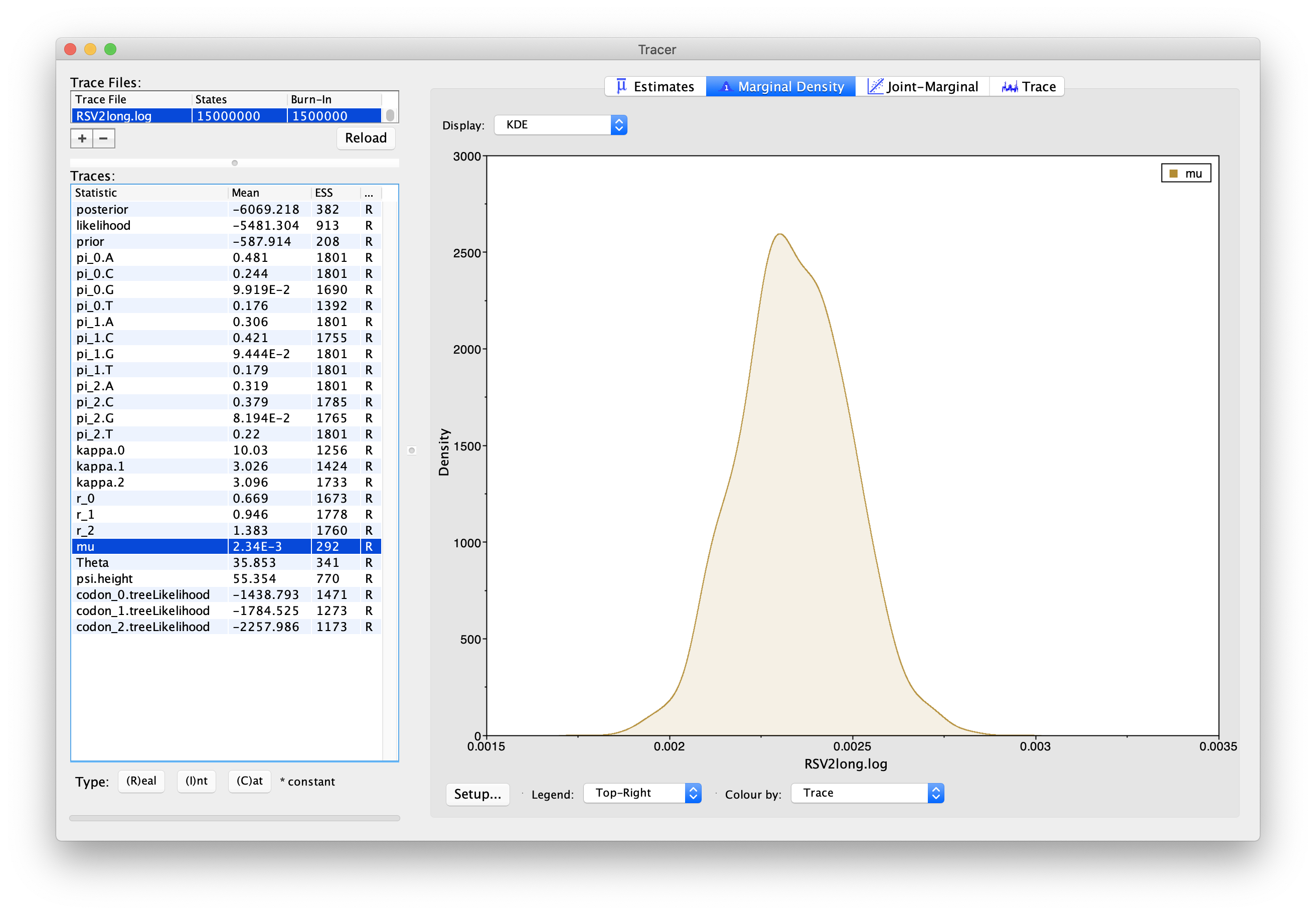
As we can see in Figure 5, the marginal
posterior probability density of μ is roughly bell-shaped.
If the curve does not look very smooth, it is because there is some
sampling noise: we could smooth it out more if we ran the MCMC chain
for longer or took more samples.
Regardless, our mean and highest posterior density interval (HPD; also
known as the credible interval) estimates should be good given the
ESSs.
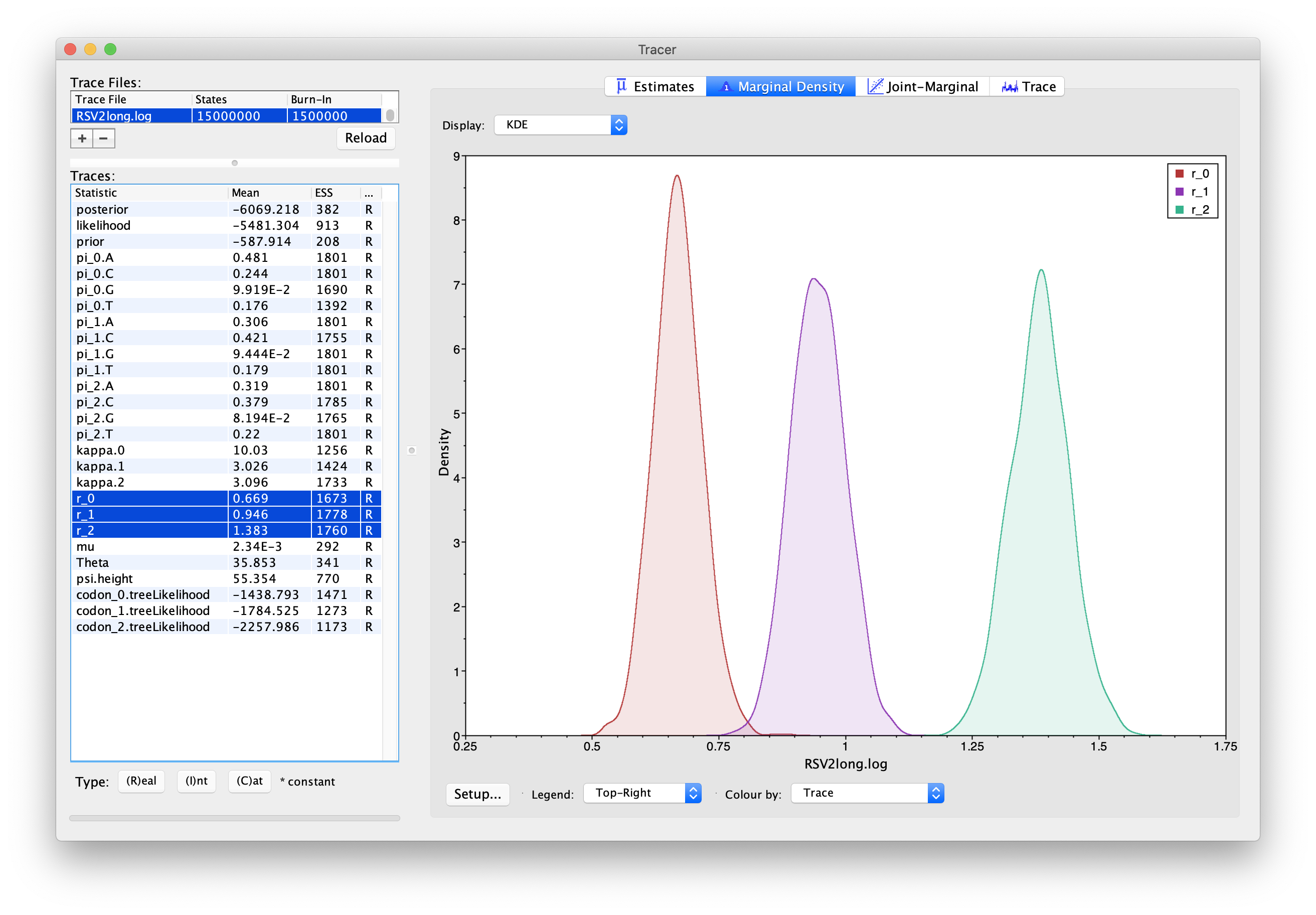
Note that you can overlay the density plots of multiple traces in order to compare them (it is up to you to determine whether they are comparable on the same axis or not). For example: select the relative rates for all three codon positions (partitions) in the left-hand panel (labelled “r_0”, “r_1” and “r_2”).
You will now see the posterior probability densities for the relative rate at all three codon positions overlaid:
Summarising the trees
Because of how peculiar and discrete tree space is, it is a bit harder
to summarize and visualize the posterior distribution over
phylogenetic trees, as compared to the mean molecular clock rate μ, for
example.
We will use a special tool for that, TreeAnnotator.
To summarize the trees logged during MCMC, we will use the CCD methods implemented in the program TreeAnnotator to create the maximum a posteriori (MAP) tree. The implementation of the conditional clade distribution (CCD) offers different parameterizations, such as CCD1, which is based on clade split frequencies, and CCD0, which is based on clade frequencies. The MAP tree topology represents the tree topology with the highest posterior probability, averaged over all branch lengths and substitution parameter values.
You need to install CCD package to make the options available in TreeAnnotator.
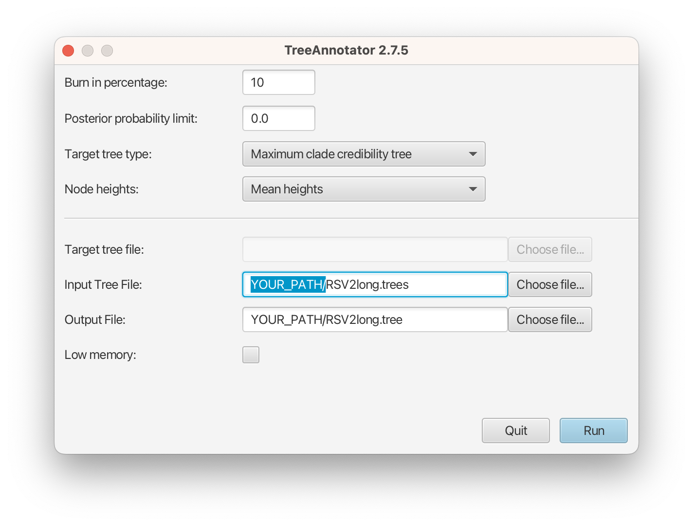
Please follow these steps after launching TreeAnnotator:
- Set 10% as the burn-in percentage;
- Select “MAP (CCD0)” as the “Target tree type”;
- For “Node heights”, choose “Common Ancestor heights”;
- Load the tree log file that BEAST 2 generated (it will end in “.trees” by default) as “Input Tree File”. For this tutorial, the tree log file is called RSV2long.trees. If you select it from the file chooser, the parent path will automatically fill in and “YOUR_PATH” in the screen shot will be that parent path.
- Finally, for “Output File”, copy and paste the input file path but replace the RSV2long.trees with RSV2long.tree. This will create the file containing the resulting MAP tree.
The image below shows a screenshot of TreeAnnotator with the necessary settings to create the summary tree. “YOUR_PATH” will be replaced to the corresponding path.
The setup described above will take the set of trees in the tree log file and summarize it with a single MAP tree using the CCD0 method. Divergence times will reflect the average ages of each node summarised by the selected method, and these times will be annotated with their 95% highest posterior density (HPD) intervals. TreeAnnotator will also display the posterior clade credibility of each node in the MAP tree. More details on summarizing trees can be found in beast2.org/summarizing-posterior-trees/.
Note that TreeAnnotator only parses a tree log file into an output text file, but the visualization has to be done with other programs (see next section).
In TreeAnnotator, mean heights are calculated as the mean MRCA time for those trees in the set where the clade is monophyletic. This approach can result in negative branch lengths in the summarized tree, if there is very low posterior support for a clade. Common ancestor heights for a clade are calculated as the average MRCA time for that clade over all trees in the set, and are not necessarily based on monophyletic clades. If you’re concerned about the differences between these two options, you can run both and compare the resulting trees.
Visualizing the trees
Summary trees can be viewed using FigTree and DensiTree, the latter being distributed with BEAST 2. In FigTree, just load TreeAnnotator’s output file as the input (if you were to load the entire tree log file, FigTree would show you each tree in the posterior individually).
After loading the summarised tree in FigTree, click on the “Trees” tab on the left-hand side, then select “Order nodes” while keeping the default ordering (“increasing”). In addition, check “Node Bars”, choosing “height_95%_HPD” for “Display”. This last step shows the estimated 95% HPD intervals for all node heights. You should end up with a tree like the one in Figure 9.

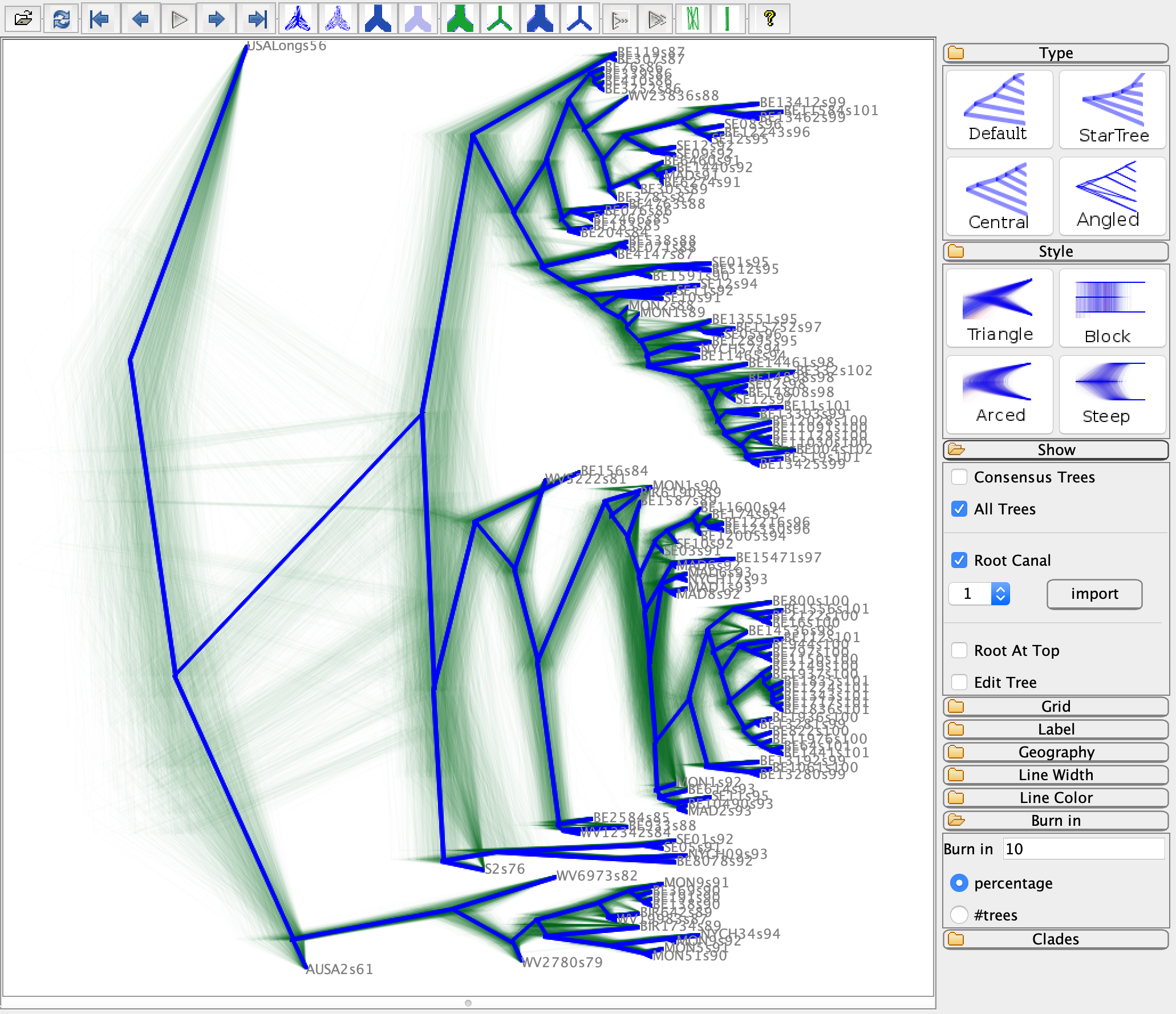
In DensiTree, load the tree log file as the input. Here, the tree in blue is the summarised tree, where the green “fuzzy” trees are all the other trees in the posterior set.
Questions
-
How can I determine if my MCMC runs have converged ?
-
What is the 95% HPD ?
-
How to compute the absolute rates of each codon given their relative rates ?
-
What is the unit of branch lengths in the time tree for this analysis ?
-
In what year did the common ancestor of all RSVA viruses sampled live ?
Programs used in this tutorial
The following software will be used in this tutorial. We also offer a Tech Help page to assist you in case you encounter any unexpected issues with certain third-party software tools.
-
Java 17 or a later version is required by LPhy Studio.
-
LPhy Studio - This software will specify, visualize, and simulate data from models defined in LPhy scripts. At the time of writing, the current version is v1.7.x. It is available for download from LPhy releases.
-
LPhy BEAST - this BEAST 2 package will convert LPhy scripts into BEAST 2 XMLs. The installation guide and usage can be found from User Manual.
-
BEAST 2 - the bundle includes the BEAST 2 program, BEAUti, DensiTree, TreeAnnotator, and other utility programs. This tutorial is written for BEAST v2.7.x or higher version. It is available for download from http://www.beast2.org. Use
Package Managerto install the required BEAST 2 packages. -
BEAST labs package - this contains some generally useful stuff used by other BEAST 2 packages.
-
BEAST feast package - this is a small BEAST 2 package which contains additions to the core functionality.
-
BEAST CCD package - Implementation of the conditional clade distribution (CCD), such as, based on clade split frequencies (CCD1) and clade frequencies (CCD0). Furthermore, point estimators based on the CCDs are implemented, which allows TreeAnnotator to produce better summary trees than via MCC trees (which is restricted to the sample).
-
Tracer - this program is used to explore the output of BEAST (and other Bayesian MCMC programs). It graphically and quantitatively summarises the distributions of continuous parameters and provides diagnostic information. At the time of writing, the current version is v1.7.x. It is available for download from Tracer releases.
-
FigTree - this is an application for displaying and printing molecular phylogenies, in particular those obtained using BEAST. At the time of writing, the current version is v1.4.x. It is available for download from FigTree releases.
XML and log files
- RSV2.xml
- RSV2.log
- RSV2.trees
- RSV2long.xml
- RSV2long.log
- RSV2long.trees
- summarised tree RSV2long.ccd0.tree
Useful links
- LinguaPhylo: https://linguaphylo.github.io
- BEAST 2 website and documentation: http://www.beast2.org/
- Join the BEAST user discussion: http://groups.google.com/group/beast-users
References
- Zlateva, K. T., Lemey, P., Vandamme, A.-M., & Van Ranst, M. (2004). Molecular evolution and circulation patterns of human respiratory syncytial virus subgroup a: positively selected sites in the attachment g glycoprotein. J. Virol., 78(9), 4675–4683.
- Zlateva, K. T., Lemey, P., Moës, E., Vandamme, A.-M., & Van Ranst, M. (2005). Genetic variability and molecular evolution of the human respiratory syncytial virus subgroup B attachment G protein. J. Virol., 79(14), 9157–9167. https://doi.org/10.1128/JVI.79.14.9157-9167.2005
- Drummond, A. J., & Bouckaert, R. R. (2014). Bayesian evolutionary analysis with BEAST 2. Cambridge University Press.
- Höhna, S., Landis, M. J., Heath, T. A., Boussau, B., Lartillot, N., Moore, B. R., Huelsenbeck, J. P., Ronquist, F. (2016). RevBayes: Bayesian phylogenetic inference using graphical models and an interactive model-specification language. Syst. Biol., 65(4), 726-736.