Model Validation
by Walter Xie, Fábio K. Mendes, and Alexei Drummond
It is very important that LPhy and LPhyBEAST developers should use the well-calibrated study to validate their new methods and models before publishing them. The study will verify whether the developed method or model satisfies its proposed functionality and also has a good accuracy.
If you are not familiar with this process and its principles, we recommend you read the BEAST 2 developer guide before starting this tutorial.
Goals
From this tutorial, you suppose to learn how to use LPhy and LPhyBEAST to validate a phylogenetic model following these steps:
- write a simple LPhy script to simulation alignments;
- run simulations using LPhyStudio;
- create BEAST 2 XML using the simulated data and specified models;
- batch processing BEAST runs;
- understand the coverage and be able to explain the test result.
A separated guide for a 5-Step pipeline in a R package will help you to summarise BEAST logs and visualise the result.
Alternatively, this tutorial can be used for other purposes of running simulations,
such as learning the scales or dynamics of a specified phylogenetic model.
Creating a LPhy script
First, we need to create a LPhy script to configure the simulations. We have provided the following script RSV2sim.lphy for this tutorial:
data {
options = {ageDirection=“forward”, ageRegex=”s(\d+)$”};
D = readNexus(file=“data/RSV2.nex”, options=options);
codon = D.charset([“3-629\3”, “1-629\3”, “2-629\3”]);
L = codon.nchar();
n = length(codon);
taxa = D.taxa();
}
model {
π ~ Dirichlet(replicates=n, conc=[2.0, 2.0, 2.0, 2.0]);
κ ~ LogNormal(sdlog=0.5, meanlog=1.0, replicates=n);
r ~ WeightedDirichlet(conc=rep(element=2.0, times=n), weights=L);
μ ~ LogNormal(meanlog=-5.0, sdlog=1.25);
Θ ~ LogNormal(meanlog=3.0, sdlog=2.0);
ψ ~ Coalescent(taxa=taxa, theta=Θ);
sim ~ PhyloCTMC(L=L, Q=hky(kappa=κ, freq=π, meanRate=r), mu=μ, tree=ψ);
}
Before you continue, please note here we want to simulate data from the exactly same model as used the time-stamped data tutorial, including all meta-data, such as dates and taxa names. It will be easy to extract these meta-data from the real data in “RSV2.nex”, but the real data is not required in the simulations. Please do not be confused with the requirements between simulations and real data analyses.
This script defines a simple 3-partition model to simulate 3 alignments using HKY with estimated frequencies and Coalescent at the constant population size. The strict molecular clock is applied. It is modified from the script in the time-stamped data tutorial. So more details about the model and priors are explained in that tutorial.
This simple model is very popular when analysing the coding genes. Each of 3 partitions can be referred to the sites at each codon position.
In the data {...} section, we are loading “RSV2.nex” to extract taxa names
and associated dates. Such information is retained in the variable taxa.
In addition, the number of partitions n and the vector of number of sites
in each partition L are also extracted from the real data.
Furthermore, In the model {...} section,
the last LPhy command sim ~ PhyloCTMC(...) explicitly instructs
not to clamp the real data codon, but to export the vector of simulated
alignments named as sim.
For the details of this model, please read the auto-generated narrative from LPhy studio, where the data section is removed.
Alternatively, you can look at another simple simulation using HKY+Coalescent. More examples are available in the examples folder in the LPhy repository.
LPhy Studio
LPhy studio is a GUI to parse your script into the probabilistic graphical models. You can download RSV2sim.lphy and load it into LPhy studio.
Now we are going to run 10 simulations.
Change the number in the text field “reps:” from 1 to 10,
then click the button “Sample”.
After switching the tab to “Variable Log”, you will see the “true” values
of these 10 simulations. Switching the tab to “Variable Log”,
you will see the “true” trees of these 10 simulations.
They can be saved into files by clicking the File menu and
Save VariableLog to File ... or Save Tree VariableLog to File ....
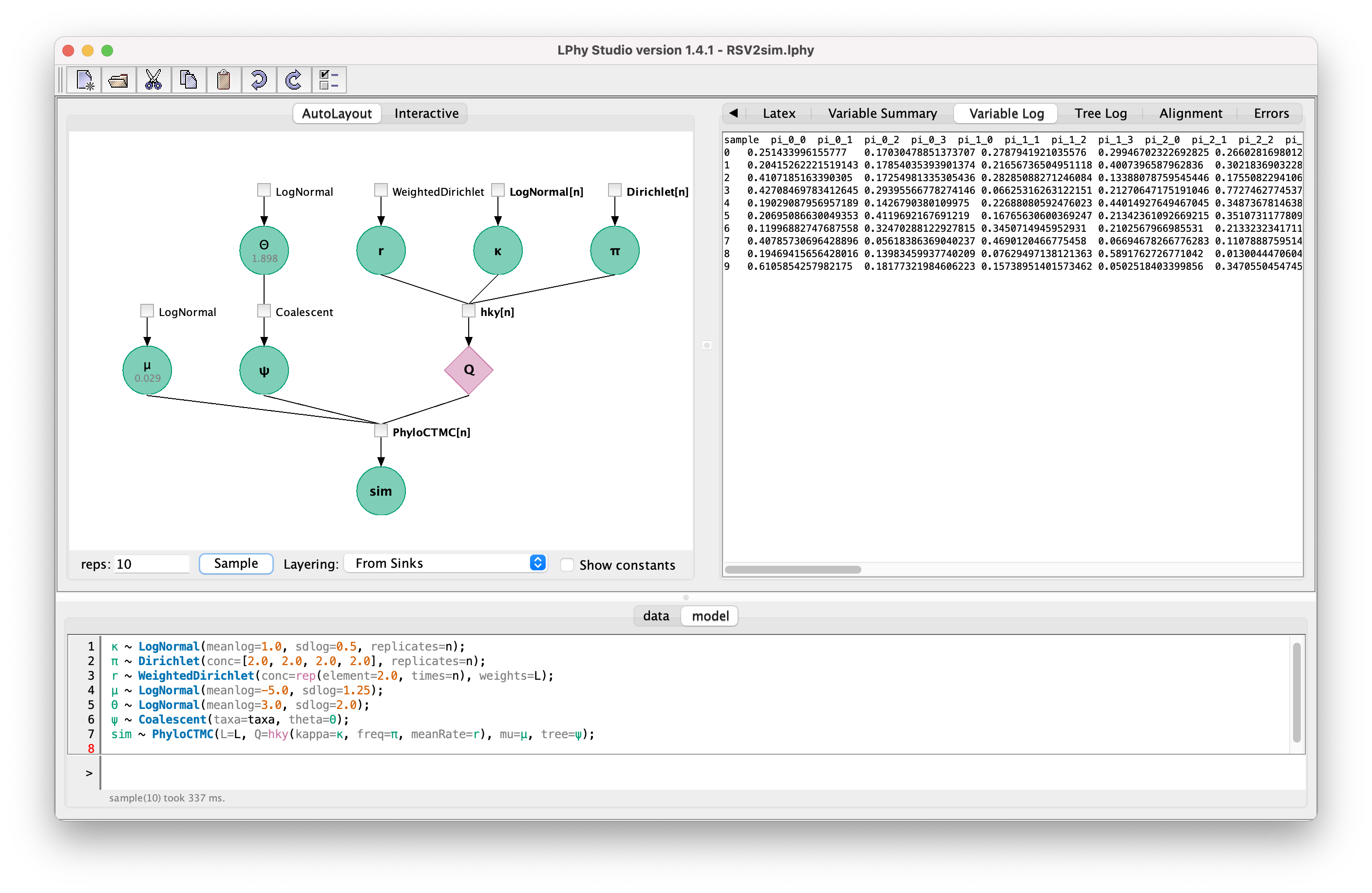
Clicking any nodes in the graph, you can view the “true” values of that variable from the last simulation.
LPhyBEAST and batch processing
LPhy studio does not have inference engine, so that we need to start LPhyBEAST to run the simulations configured by the LPhy script, and create BEAST 2 XMLs based on these simulation results. These XMLs will contain the simulated alignments and the models specified by your script.
Run the following command in the terminal to complete this task:
$LPhyBEAST -r 110 -l 50000000
           -o $MY_XML_FOLDER/al2.xml
           $LPHY_PATH/tutorials/RSV2sim.lphy
$LPhyBEAST supposes to be the command to start LPhyBEAST.
The rests are the arguments to indicate creating 110 BEAST XMLs with a file steam
“al2”, and saving all XMLs to the folder $MY_XML_FOLDER (e.g. “/home/…/WorkSpace/xmls/”).
The absolute path must be used for both $MY_XML_FOLDER and $LPHY_PATH.
This will also create extra logs containing “true” values and “true” trees. In the end, we will check ESS and only select 100 results to calculate the coverage. Those 10 extra simulation results will be used to replace any of 100 results having low ESS (<200) if there is any. The processing detail is explained in the guide of 5-Step Pipeline,
The benefit of using -r is that LPhyBEAST will create the XMLs
whose log file names are distinct to one another.
Their names are concatenated by the same file steam and index numbers
and separated by an underscore.
For example, in the generated al2_0.xml, the log file name is al2_0.log
and tree log file name is al2_0.trees.
So you do not need to worry about the overwriting problem, when you run all XMLs
in the same folder.
More usage details are available here.
BEAST runs
The following Linux commands will run all XMLs in the same folder,
where $BEAST2 is the folder containing BEAST 2 package.
for xml in *.xml; do
    echo "run $xml"
    $BEAST2/bin/beast -beagle_SSE $xml
done
It will take a while if not using a HPC (High Performance Computing) cluster. But you can download all required logs (we do not need BEAST tree logs) for the next step from the LPhy website repository. They are compressed into several *.tar.gz files. You need to extract the logs into the same folder using the Linux command below:
ls *.gz | xargs -n1 tar -xzf
Coverage
The results can be summarised by
5-Step Pipeline,
which will produce intermediate *.tsv files containing the statistic summaries
in each step.
It can create the figure to report coverage, for example, the coverage of the mutation rate parameter “mu” looks like:
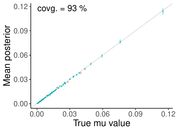
The x-axis represents the “true” value of “mu”, which has been created by LPhy during the simulation. The y-axis represents the posterior of “mu” sampled by BEAST 2. There are 100 dots and bars in this graph. Each bar is the 95% HPD interval of the posterior samples of “mu” in one simulation, and the dot inside the bar is the mean.
If the “true” value falls into the 95% HPD interval, the result will be valid, and then the bar will be coloured as blue. Otherwise, the validation will fail, and the bar is red. There are 93 simulations having the “true” value falling into the 95% HPD interval for “mu”, so the coverage will be 93%.
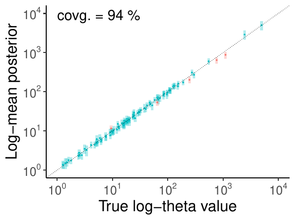
Sometimes, the log-scale is required, such as the population size “theta”:
A good coverage for all parameters from model validation is the confirmation of a successfully validated method or model.
If the coverage is low, before you make a conclusion that your method or model would have something wrong, you should check whether the posteriors are converged. It is not solid evidence to prove the convergence, even though the ESSs of every parameters are greater than 200.