Ancestral Reconstruction using Discrete Phylogeography

If you haven’t installed LPhy Studio and LPhyBEAST yet, please refer to the User Manual for their installation. Additionally, this tutorial requires other third-party programs, which are listed below under the section Programs used in this tutorial.

This tutorial guides you through a discrete phylogeography analysis of a H5N1 epidemic in South China. The analysis will use the model developed by Lemey et al., 2009 that implements ancestral reconstruction of discrete states (locations) in a Bayesian statistical framework, and employs the Bayesian stochastic search variable selection (BSSVS) to identify the most plausible description of the phylogeographic diffusion process.

The additional benefit in using this model is that we can summarise the phylogeographic inferences from an analysis, and use a virtual globe software to visualise the spatial and temporal information.

The NEXUS alignment

The data is available in a file named H5N1.nex. If you have installed LPhy Studio, you don’t need to download the data separately. It comes bundled with the studio and can be accessed in the “tutorials/data” subfolder within the installation directory of LPhy Studio.

This alignment is a subset of original dataset Wallace et al., 2007, and it consists of 43 influenza A H5N1 hemagglutinin and neuraminidase gene sequences. These sequences were isolated from a diverse range of hosts over the period from 1996 to 2005 across various sampling locations.

Loading the script “h5n1” to LPhy Studio

To get started, launch LPhy Studio. To load the script into LPhy Studio, click on the File menu and hover your mouse over Tutorial scripts. A child menu will appear, and then select the script h5n1.

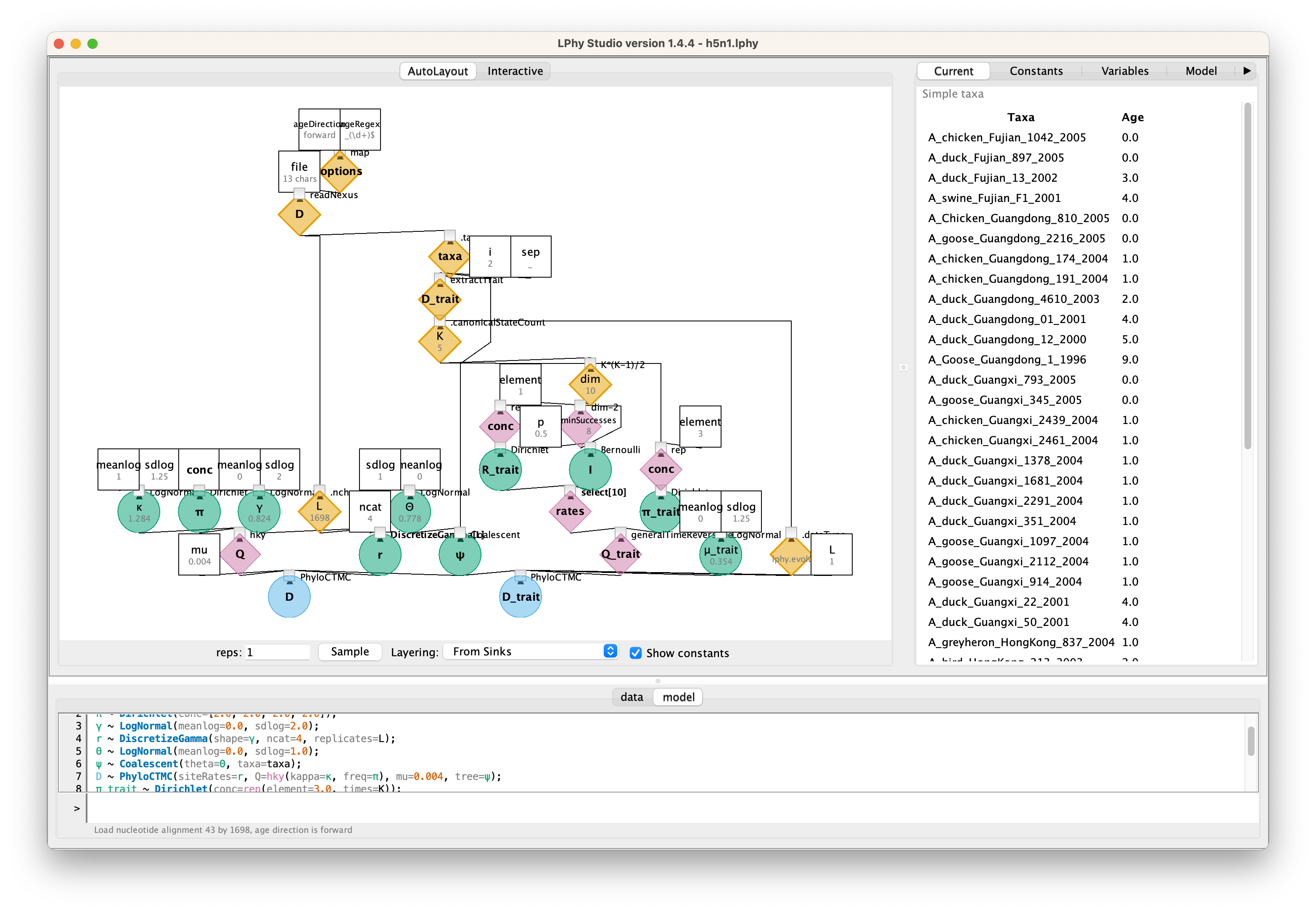
The probabilistic graphical model will be visualised on the left panel. By clicking on the graphical components, you can view their current values displayed in the right-side panel titled Current. You can also switch the view to show the script after clicking on the tab Model. The next tab, Narrative, will display an auto-generated narrative using natural language to describe the models with citations. This narrative can serve as the foundation for manuscript method sections.

If you are not familiar with LPhy language, we recommend reading the language features before getting started.

Code

data {
  options = {ageDirection="forward", ageRegex="_(\d+)$"};
  D = readNexus(file="data/H5N1.nex", options=options);
  L = D.nchar();
  taxa = D.taxa();
  D_trait = extractTrait(taxa=taxa, sep="_", i=2);
  K = D_trait.canonicalStateCount();
  dim = K*(K-1)/2;
  dataType = D_trait.dataType();
}
model {
  π ~ Dirichlet(conc=[2.0, 2.0, 2.0, 2.0]);
  κ ~ LogNormal(meanlog=1.0, sdlog=1.25);
  γ ~ LogNormal(meanlog=0.0, sdlog=2.0);
  r ~ DiscretizeGamma(shape=γ, ncat=4, replicates=L);
  Θ ~ LogNormal(meanlog=0.0, sdlog=1.0);
  ψ ~ Coalescent(taxa=taxa, theta=Θ);
  D ~ PhyloCTMC(Q=hky(kappa=κ, freq=π), mu=0.004, siteRates=r, tree=ψ);
  π_trait ~ Dirichlet(conc=rep(element=3.0, times=K));
  I ~ Bernoulli(minSuccesses=dim-2, p=0.5, replicates=dim);
  R_trait ~ Dirichlet(conc=rep(element=1.0, times=dim));
  Q_trait = generalTimeReversible(rates=select(x=R_trait, indicator=I), freq=π_trait);
  μ_trait ~ LogNormal(meanlog=0, sdlog=1.25);
  D_trait ~ PhyloCTMC(L=1, Q=Q_trait, dataType=dataType, mu=μ_trait, tree=ψ);
}

Graphical Model

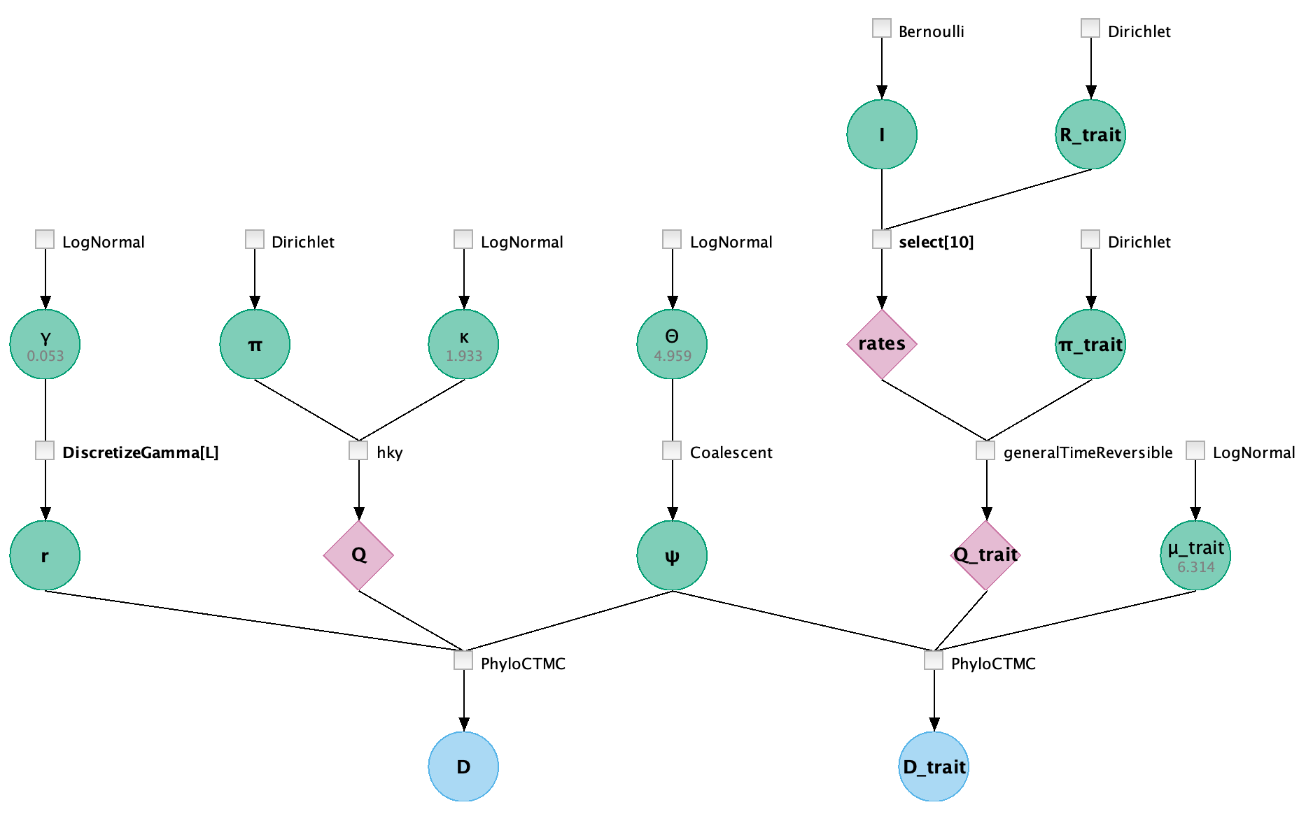
Data block

In the data block, we begin by defining an option to extract the sample times from the taxa labels using a regular expression _(\d+)$, and we treat those times as dates (i.e., moving forward in time). For instance, the taxon “A_chicken_Fujian_1042_2005” will yield the year 2005, making the age of this tip 0 since 2005 is the latest year among these samples. Clicking on the orange diamond labeled “taxa”, you can see all taxa along with their ages, which have been converted from the years extracted from their labels. If it is not in the probabilistic graphical model, please select the checkbox Show constants to display the full model.

Next, we read the file “H5N1.nex” and load it into an alignment D, using the previously defined options. Following that, we assign the constant L to represent the number of sites in alignment D, and we retrieve the vector of taxa names from the alignment D.

The line using the function extractTrait extracts the locations from the taxa names by splitting the string by “_” and taking the 3rd element (where i starts at 0). This code creates a trait alignment D_trait containing the locations mapped to each taxon. Then the method canonicalStateCount() counts the number of unique canonical states (locations) in the trait alignment D_trait and assigns this number to the constatnt K. This method excluds ambiguous states. The constant dim used as the dimension for sampling discrete traits is computed from K.

Model block

In the model block, we have mixed two parts. The first part is modeling evolutionary history and demographic structure based on a nucleotide alignment, and the second part is defining how to sample the discrete states (locations) from the phylogeny shared with the 1st part.

Coalescent based phylogenetic model

The canonical model in the first part of this analysis includes the following parameter distributions:

Dirichlet prior on, π, the equilibrium nucleotide frequencies (with 4 dimensions, one for each nucleotide);
LogNormal prior on, κ, the transition/transversion ratio;
LogNormal prior on, γ, the shape parameter of discretize Gamma;
Discretized gamma prior on, r, the vector of site rates with a rate for each site in the alignment;
LogNormal prior on, Θ, the effective population size;
Coalescent (constant-size) prior on, ψ, the time-scaled phylogenetic tree which is scaled according to the unit of sampling time associated with taxa. The time unit in this data is years.

Finially, the phylogenetic continuous-time Markov chain distribution, PhyloCTMC, utilizes the instantaneous rate matrix Q retured from a deteminstic function hky, the site rates r, and the simulated Coalescent tree ψ as inputs, along with a fixed value of 0.004 for the mutation rate, to generate the alignment D.

For more details, please read the auto-generated narrative from LPhy Studio.

Geographic Model

The next part is the geographic model. In the discrete phylogeography, the probability of transitioning to a new location through the time is computed by

\[P(t) = e^{\Lambda t}\]

where $\Lambda$ is a $ K \times K $ infinitesimal rate matrix, and $K$ is the number of discrete locations (i.e. 5 locations here). Then,

\[\Lambda = \mu S \Pi\]

where $\mu$ is an overall rate scalar, $S$ is a $ K \times K $ matrix of relative migration rates, and $\Pi = diag(\pi)$ where $\pi$ is the equilibrium trait frequencies. After the normalization, $\mu$ measures the number of migration events per unit time $t$. The detail is explained in Lemey et al., 2009.

So, assuming migration to be symmetric in this analysis:

We define a vector variable R_trait with the length of $ \frac{K \times (K-1)}{2} $ to store the off-diagonal entries of the unnormalised $S$, which is sampled from a Dirichlet distribution.
A boolean vector I with the same length determines which infinitesimal rates are zero, and it is sampled from the vectorized function Bernoulli using the keyword replicates. This along with the deterministic function select implements the Bayesian stochastic search variable selection (BSSVS).
The base frequencies π_trait are sampled from a Dirichlet distribution.
The deteminstic function generalTimeReversible takes relative rates filtered by select, which selects a value if the indicator is true or returns 0 otherwise, along with base frequencies to produce the general time reversible rate matrix Q_trait.
The migration rate, μ_trait, is sampled from a LogNormal distribution.

In the end, the 2nd PhyloCTMC takes the instantaneous rate matrix Q_trait, the data type from the clamped alignment D_trait imported in the data block, the migration rate μ_trait, the same tree ψ sampled from the 1st part of this model as inputs, to simulate the location alignment D_trait whose supposes to have only one site.

As you have noticed, there are two D_trait in this script, one is in the data block, the other is in the model block. This is called data clamping. The detail can be refered to either the section “2.1.11 Inference and data clamping” in the LPhy paper or visit the LPhy language features page.

Producing BEAST XML using LPhyBEAST

BEAST 2 retrieves the data and model specifications from a XML file. One of our goals with LPhy is to make configuring Bayesian phylogenetic analysis as painless, clear and precise as possible. In order to achieve that, we will utilize an additional companion application called LPhyBEAST, which acts as a bridge between the LPhy script and the BEAST 2 xml. It is distributed as a BEAST 2 package, please follow the instruction to install it.

To run LPhyBEAST and produce a BEAST 2 xml, you need to use the terminal and execute the script lphybeast. The LPhyBEAST usage can help you get started. In our h5n1.lphy script, the alignment file is assumed to be located under the subfolder tutorials/data/. To generate the XML, navigate to the tutorials folder where LPhy is installed, and run the following command in your terminal. After it completes, check the message in the end to find the location of the generated XML file.

For example, on a Mac, after replacing all “x” with the correct version number, you can execute the following lphybeast command in the terminal to launch LPhyBEAST:

# go to the folder containing lphy script
cd /Applications/lphystudio-1.x.x/tutorials
# run lphybeast
'/Applications/BEAST 2.7.x/bin/lphybeast' -l 3000000 h5n1.lphy

If you are not familiar with inputting valid paths in the command line, here is our Tech Help that may help you.

For Windows users, please note that “C:\Program Files” is usually a protected directory. However, you can copy the “examples” and “tutorials” folders with “data” into your “Documents” folder and work in that location to avoid any permission issues. Alternatively, run lphybeast.bat on a Windows terminal like this:

# go to the subfolder containing lphy script
cd "C:\Users\<YourUserName>\Documents\tutorials"
# run lphybeast
"C:\Program Files\BEAST2.7.x\bat\lphybeast.bat" -l 3000000 h5n1.lphy

Please note that the single or double quotation marks ensure that the whitespace in the path is treated as valid.

The -l option allows you to modify the MCMC chain length in the XML, which is set to the default of 1 million.

After LPhyBEAST completes the run, it will print a location information for the BEAST 2 XML at the end of the message. For example, on a Mac system:

INFO: Save BEAST 2 XML to /Applications/lphystudio-1.4.4/tutorials/h5n1.xml

Running BEAST

After LPhyBEAST generates a BEAST 2 .xml file (e.g., h5n1.xml), we can use BEAST 2 to load it and start the inferential MCMC analysis. BEAST 2 will write its outputs to disk into specified files in the XML, and also output the progress of the analysis and some summaries to the screen.

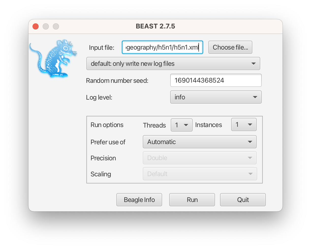
The h5n1.xml is also provided as an additional resource, in case you need to use it for your analysis.

                        BEAST v2.7.5, 2002-2023
             Bayesian Evolutionary Analysis Sampling Trees
                       Designed and developed by
 Remco Bouckaert, Alexei J. Drummond, Andrew Rambaut & Marc A. Suchard
                                    
                   Centre for Computational Evolution
                         University of Auckland
                       r.bouckaert@auckland.ac.nz
                        alexei@cs.auckland.ac.nz
                                    
                   Institute of Evolutionary Biology
                        University of Edinburgh
                           a.rambaut@ed.ac.uk
                                    
                    David Geffen School of Medicine
                 University of California, Los Angeles
                           msuchard@ucla.edu
                                    
                      Downloads, Help & Resources:
                           http://beast2.org/
                                    
  Source code distributed under the GNU Lesser General Public License:
                   http://github.com/CompEvol/beast2
                                    
                           BEAST developers:
   Alex Alekseyenko, Trevor Bedford, Erik Bloomquist, Joseph Heled, 
 Sebastian Hoehna, Denise Kuehnert, Philippe Lemey, Wai Lok Sibon Li, 
Gerton Lunter, Sidney Markowitz, Vladimir Minin, Michael Defoin Platel, 
          Oliver Pybus, Tim Vaughan, Chieh-Hsi Wu, Walter Xie
                                    
                               Thanks to:
          Roald Forsberg, Beth Shapiro and Korbinian Strimmer

Random number seed: 1690144368524

    ...

    ...
        2850000     -5948.3636     -5828.3061      -120.0575         0.3462         0.1935         0.2107         0.2494         8.5222         0.4026         7.3155         0.1285         0.1858         0.3281         0.2090         0.1483              1              0              0              1              1              0              1              1              1              1         0.2497         0.0028         0.0442         0.0361         0.2116         0.1654         0.0968         0.0853         0.0954         0.0121         0.9876 58s/Msamples
        3000000     -5943.2773     -5824.1062      -119.1710         0.3390         0.1887         0.2230         0.2492         7.4086         0.3509         8.6087         0.2398         0.2185         0.1255         0.2641         0.1518              1              0              1              1              1              1              0              1              1              0         0.1512         0.0134         0.0604         0.2013         0.2678         0.0532         0.0540         0.1006         0.0975 4.341722237E-5         0.3844 58s/Msamples

Operator                                                                        Tuning    #accept    #reject      Pr(m)  Pr(acc|m)
beast.base.inference.operator.BitFlipOperator(I.bitFlip)                             -      41315      88745    0.04340    0.31766 
beast.base.inference.operator.DeltaExchangeOperator(R_trait.deltaExchange)     0.59941      15523     105271    0.04031    0.12851 
ScaleOperator(Theta.scale)                                                     0.45689       7406      18797    0.00866    0.28264 
ScaleOperator(gamma.scale)                                                     0.40909       6810      19143    0.00866    0.26240 
ScaleOperator(kappa.scale)                                                     0.54422       7482      18572    0.00866    0.28717 
ScaleOperator(mu_trait.scale)                                                  0.28543       8107      17702    0.00866    0.31412 
beast.base.inference.operator.UpDownOperator(mu_traitUppsiDownOperator)        0.90177      35457     326061    0.12047    0.09808 Try setting scaleFactor to about 0.95
beast.base.inference.operator.DeltaExchangeOperator(pi.deltaExchange)          0.06476       9663      46498    0.01868    0.17206 
beast.base.inference.operator.DeltaExchangeOperator(pi_trait.deltaExchange)    0.68115       8541      59870    0.02285    0.12485 
Exchange(psi.narrowExchange)                                                         -      60639     294971    0.11850    0.17052 
ScaleOperator(psi.rootAgeScale)                                                0.75330       3290      22690    0.00866    0.12664 
ScaleOperator(psi.scale)                                                       0.90540      35602     320167    0.11850    0.10007 
SubtreeSlide(psi.subtreeSlide)                                                 0.92349      67477     287672    0.11850    0.19000 
Uniform(psi.uniform)                                                                 -     148469     206550    0.11850    0.41820 
Exchange(psi.wideExchange)                                                           -       1643     354433    0.11850    0.00461 
WilsonBalding(psi.wilsonBalding)                                                     -       2047     353388    0.11850    0.00576 

     Tuning: The value of the operator's tuning parameter, or '-' if the operator can't be optimized.
    #accept: The total number of times a proposal by this operator has been accepted.
    #reject: The total number of times a proposal by this operator has been rejected.
      Pr(m): The probability this operator is chosen in a step of the MCMC (i.e. the normalized weight).
  Pr(acc|m): The acceptance probability (#accept as a fraction of the total proposals for this operator).


Total calculation time: 176.085 seconds
End likelihood: -5943.277342794984
Done!

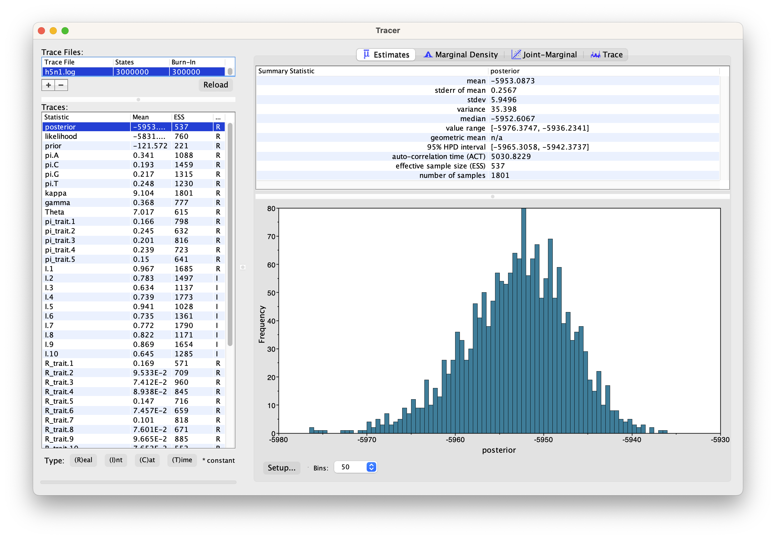
Analysing the BEAST output

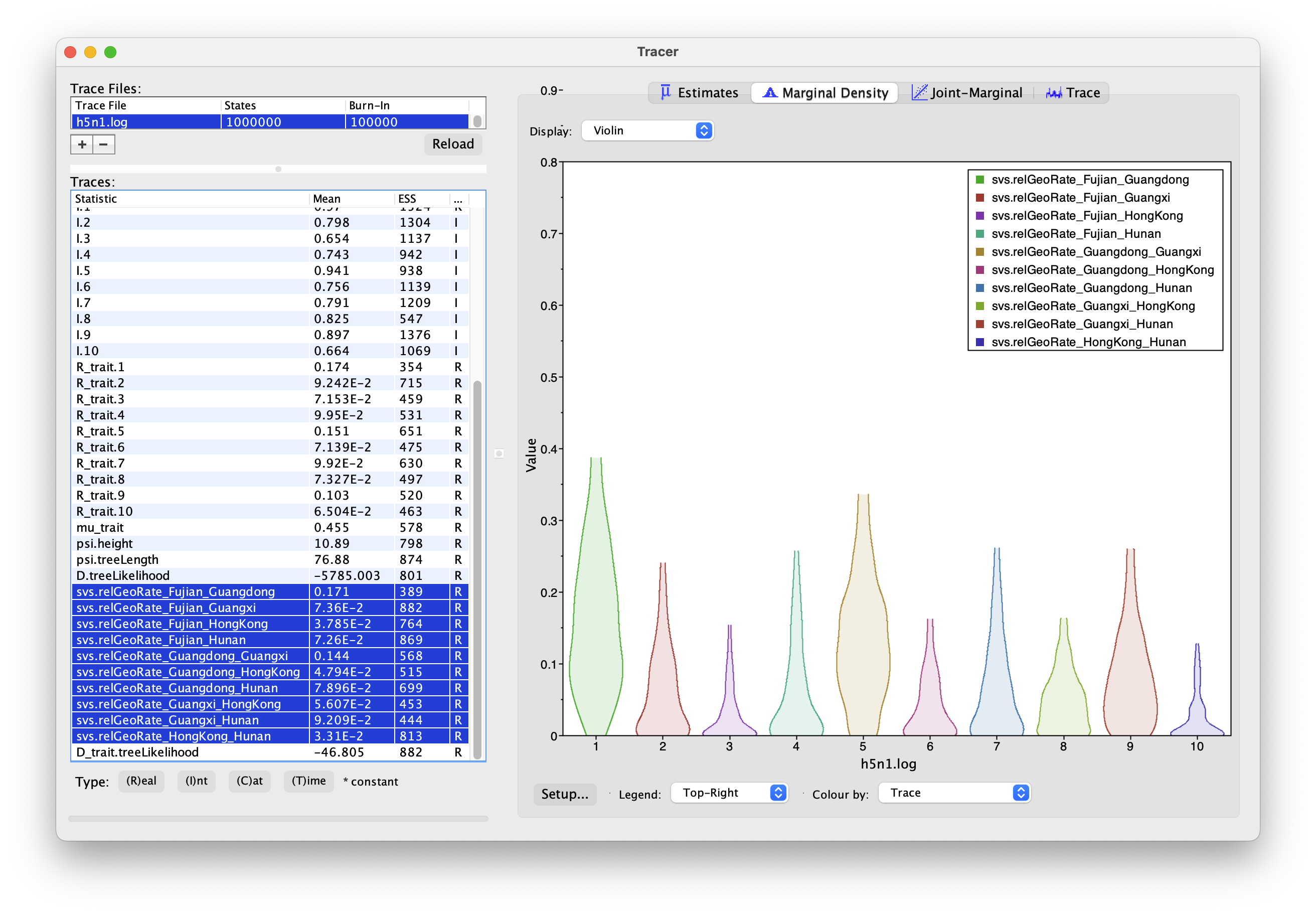
Run the program called Tracer to analyze the output of BEAST. When the main window has opened, choose Import Trace File... from the File menu and select the file that BEAST has created called h5n1.log. You should now see a window like in Figure 3.

Figure Figure 3: A screenshot of Tracer.

Remember that MCMC is a stochastic algorithm so the actual numbers will not be exactly the same. On the left hand side is a list of the different quantities that BEAST has logged. There are traces for the posterior (this is the log of the product of the tree likelihood and the prior probabilities), and the continuous parameters. Selecting a trace on the left brings up analyses for this trace on the right hand side depending on tab that is selected. When first opened, the “posterior”” trace is selected and various statistics of this trace are shown under the Estimates tab. In the top right of the window is a table of calculated statistics for the selected trace.

Tracer will plot a (marginal posterior) distribution for the selected parameter and also give you statistics such as the mean and median. The 95% HPD lower or upper stands for the highest posterior density interval and represents the most compact interval on the selected parameter that contains 95% of the posterior probability. It can be thought of as a Bayesian analog to a confidence interval.

In the implemented phylogeographic model, the rate matrix is symmetric, meaning that a relative migration rate between two locations solely represents a numerical value without implying any direction. Consequently, for 5 locations, there are only 10 relative migration rates, as illustrated in Figure 4.

DensiTree — Figure 4: The posterior of relative migration rates between two locations.

The h5n1.log is also provided as an additional resource, in case you need to use it for your analysis.

Summarizing posterior trees

To summarize the trees logged during MCMC and create a maximum clade credibility (MCC) tree, launch the program TreeAnnotator and follow these steps:

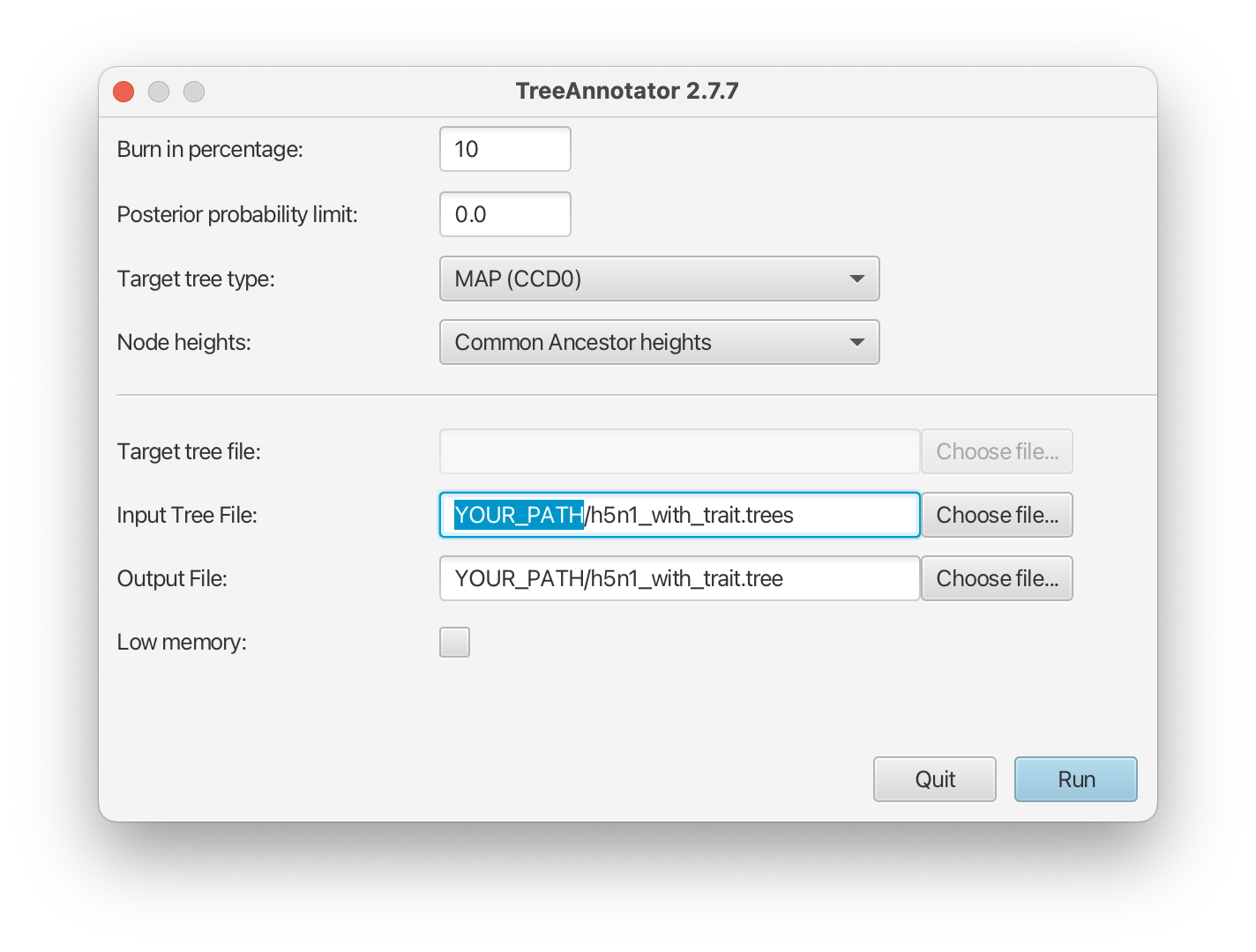
Set 10% as the burn-in percentage;
Select “Maximum clade credibility tree” as the “Target tree type”;
For “Node heights”, choose “Mean heights”;
Load the tree log file that BEAST 2 generated (it will end in “.trees” by default) as “Input Tree File”. For this tutorial, the tree log file is called h5n1_with_trait.trees. If you select it from the file chooser, the parent path will automatically fill in and “YOUR_PATH” in the screen shot will be that parent path.
Finally, for “Output File”, copy and paste the input file path but replace the h5n1_with_trait.trees with h5n1_with_trait.tree. This will create the file containing the resulting maximum clade credibility tree.

The image below shows a screenshot of TreeAnnotator with the necessary settings to create the summary tree. “YOUR_PATH” will be replaced to the corresponding path.

The setup described above will take the set of trees in the tree log file and summarize it with a single MCC tree. The MCC tree is the tree that has the largest clade probability product across all nodes. Divergence times will reflect the mean ages of each node, and these times will be annotated with their 95% highest posterior density (HPD) intervals. TreeAnnotator will also display the posterior clade credibility of each node in the MCC tree. More details on summarizing trees can be found in beast2.org/summarizing-posterior-trees/.

Note that TreeAnnotator only parses a tree log file into an output text file, but the visualization has to be done with other programs (see next section).

Both h5n1_with_trait.trees and h5n1_with_trait.tree are provided as an additional resource, in case you need to use it for your analysis.

Distribution of root location

When you open the summary tree with locations h5n1_with_trait.tree in a text editor, and scroll to the most right and locate the end of the tree definition, you can see the set of meta data for the root. Looking for the last entries of location.set and location.set.prob, you might find something like this:

location.set = {Guangdong,HongKong,Hunan,Guangxi,Fujian}
location.set.prob = {0.1793448084397557,0.5985563575791227,0.03997779011660189,0.1265963353692393,0.0555247084952804}

This means that we have the following distribution for the root location:

Location	Probability
Guangdong	0.1793448084397557
HongKong	0.5985563575791227
Hunan	0.03997779011660189
Guangxi	0.1265963353692393
Fujian	0.0555247084952804

This distribution shows that the 95% HPD consists of all locations except Hunan, with a strong indication that HongKong might be the root with over 59% probability. It is quite typical that a lot of locations are part of the 95% HPD in discrete phylogeography.

Viewing the Location Tree

We can visualise the tree in a program called FigTree. There is a bug to launch the Mac version of FigTree v1.4.4. Feel free to visit our Tech Help page if you encounter any difficulties or need assistance.

Lauch the program, and follow the steps below:

Open the summary tree file h5n1_with_trait.tree by using the Open... option in the File menu;
After the tree appears, expend Appearance and choose Colour by location;
Additionally, you can adjust the branch width based on the posterior support of estimated locations by selecting Width by location.prob.
Gradually increasing the Line Weight can make the branch widths vary more significantly based on their posterior supports.
To add a legend, tick Legend and choose location from the drop-down list of Attribute;
If you want to see the x-axis scale, you can tick Scale Axis, expend it and uncheck the option Show grid.

You should end up with something like Figure 6

MCC tree — Figure 6: Figtree representation of the summary tree. Branch colours represent location and branch widths posterior support for the branch.

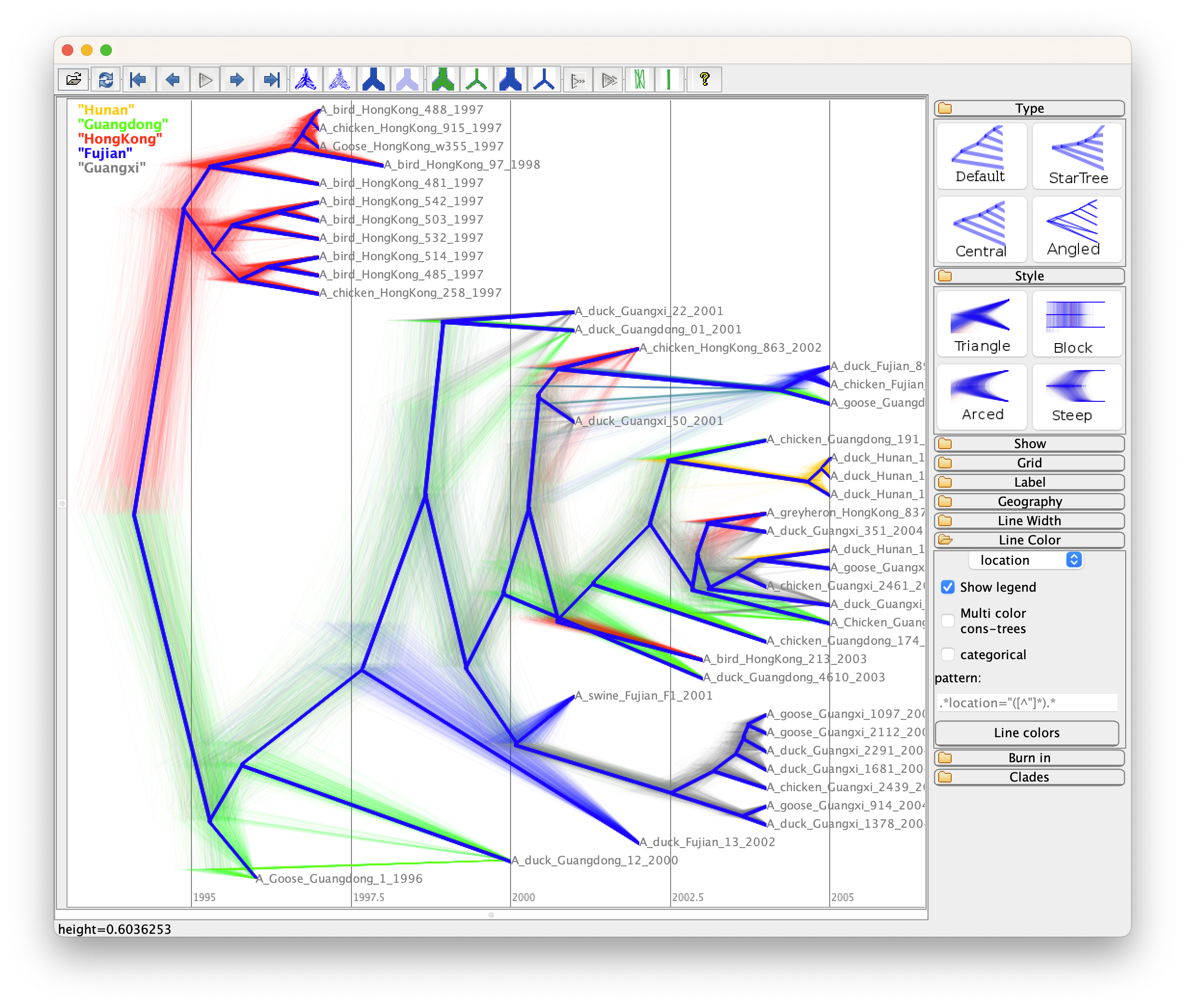
Alternatively, you can use DensiTree to visulize the set of posterior trees
and set it up as follows:

Use the Load option in the File menu to load the trees from h5n1_with_trait.trees (note this is NOT the summary tree, but the complete set);
Click Show to choose Root Canal tree to guide the eye;
Click Grid to choose Full grid option, type “2005” in the Origin text field which is the year, and tick Reverse to show the correct time scale; You also can reduce the Digits to 0 which will rounding years in the x-axis (i.g. 2005, instead of 2005.22);
Go to Line Color, you can colour branches by location and tick Show legend.

The final image look like Figure 7.

Bonus sections

The number of estimated transitions

To visualize how the location states change through the phylogeny, you can use the StateTransitionCounter tool, which counts the number of branches in a tree or a set of trees that have a certain state at the parent and another state at the node.

To use StateTransitionCounter, first, install the Babel package and then run the tool through the BEAST application launcher. The command below will generate the output file stc.out containing all counts from the logged posterior trees h5n1_with_trait.trees, after removing 10% burn-in.

$BEAST2_PATH/bin/applauncher StateTransitionCounter -burnin 10 -in h5n1_with_trait.trees -tag location -out stc.out

Make sure you have installed the latest versions of Babel (>= v0.4.x) and BEASTLabs (>= v2.0.x) to ensure smooth execution.

Next, we will use R to plot the histogram based on the summary in stc.out. If you encounter any issues generating it, you can download a prepared file stc.out. Additionally, download the script PlotTransitions.R, which contains functions to parse the file and plot the histograms. Before running the script, make sure you have installed the R packages ggplot2 and tidyverse.

Run the following scripts in R, where R_SRC_PATH is the folder containing R code, and YOUR_WD is the folder containing the stc.out file:

setwd(R_SRC_PATH)
source("PlotTransitions.R")
setwd(YOUR_WD)

# stc.out must be in YOUR_WD
stc <- parseTransCount(input="stc.out", pattern = "Histogram", target="Hunan")
# only => Hunan
p <- plotTransCount(stc$hist[grepl("=>Hunan", stc$hist[["Transition"]]),], 
        colours = c("Fujian=>Hunan" = "#D62728", "Guangdong=>Hunan" = "#C4C223", 
                    "Guangxi=>Hunan" = "#60BD68", "HongKong=>Hunan" = "#1F78B4"))
ggsave( paste0("transition-distribution-hunan.png"), p, width = 6, height = 4) 

The stc file contains a statistical summary of the estimated transition counts related to the target location, which is Hunan, and a table of the actual counts. To plot a simple graph, we will pick up the transitions to Hunan in the next command and then save the graph as a PNG file. The counts will be normalized into probabilities.

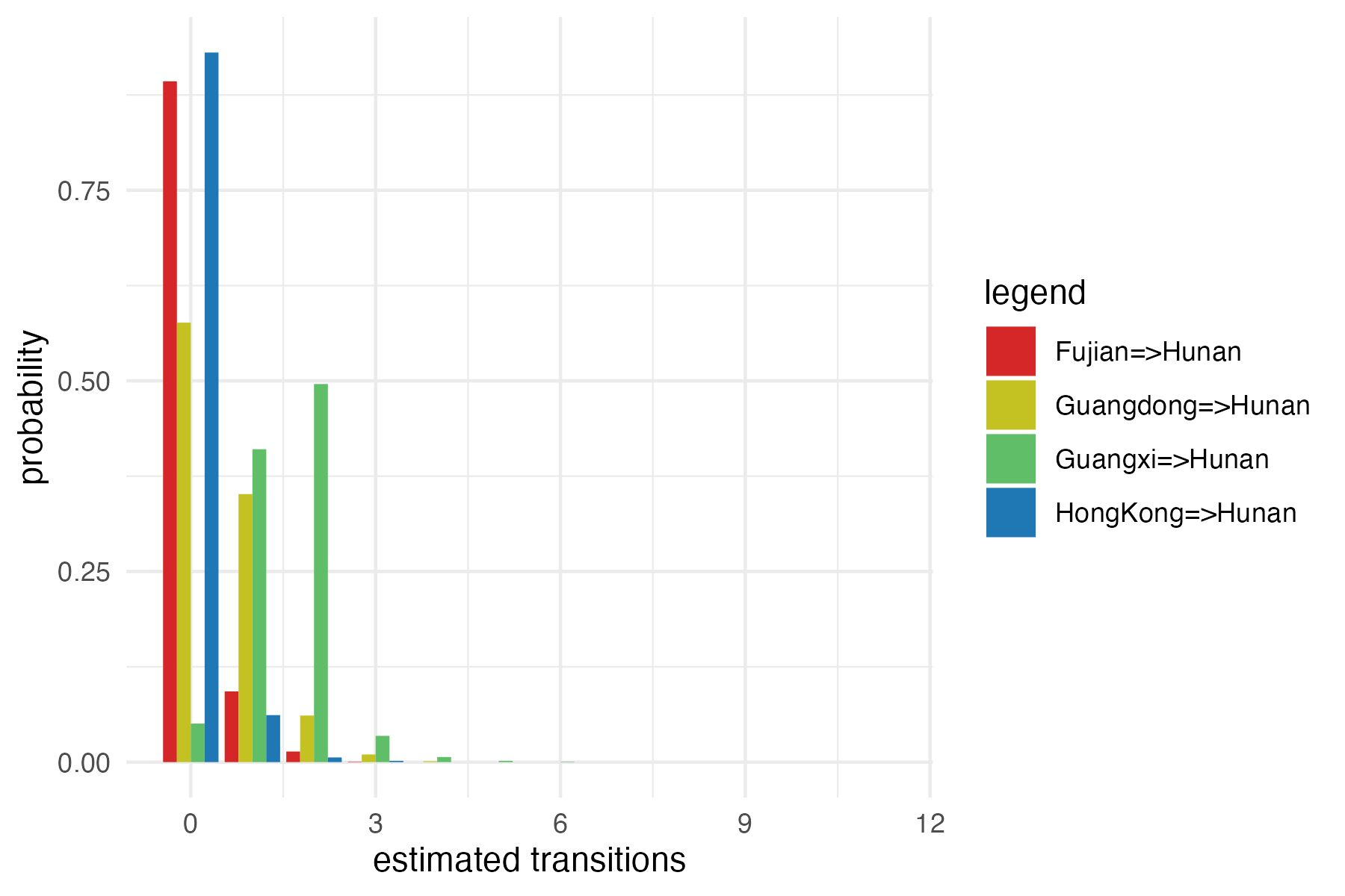
The x-axis represents the number of estimated transitions in all migration events from one particular location to another, separated by “=>”, and the y-axis represents the probability, which is normalized from the total counts. From the graph, we can observe that “Guangxi => Hunan” (in blue) has a higher probability than other migration events. This type of visualization quantifies the uncertainty in how the disease (H5N1) spreads between locations of interest, as simulated from your model and given the data. For more details and visualizations, you can refer to the work of Douglas et. al. 2020.

Visualizing phylogeographic diffusion

To analyze and visualize phylogeographic reconstructions resulting from Bayesian inference of spatio-temporal diffusion based on the Bielejec et al., 2011 method, we can use a software called spread.

Please note it requires Java 1.8. If you run into any issues or need support, don’t hesitate to check out our Tech Help page.

We recommend to download the .jar file from the Spread website, and follow the steps below:

Start the spread application by using the command java -jar SPREADv1.0.7.jar.
Select the Open button in the panel under Load tree file.
Choose the summary tree file h5n1_with_trait.tree`.
Change the State attribute name to the name of the trait, which is location in this analysis.
Click the Setup button to edit altitude and longitude for the locations. You can also load this information from a tab-delimited file, and a prepared file locationCoordinates_H5N1.txt is also available. Remeber to click Done button to save the information into spread.
Change the Most recent sampling date to 2005.
Open the Output tab in the left-hand side panel, and then choose where to save the KML file (default is output.kml).
Click the Generate button to create the KML file.

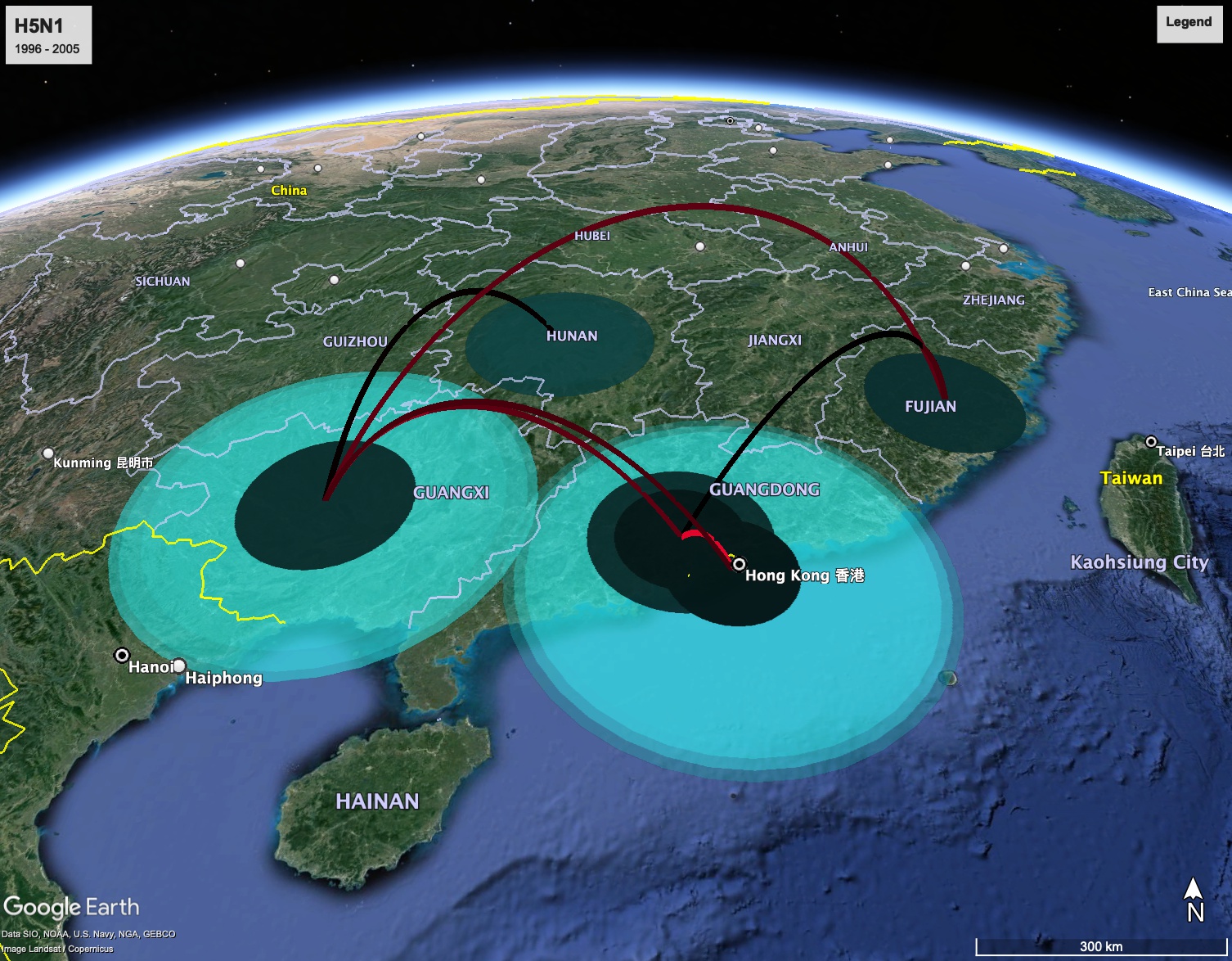
The world map with the tree superimposed onto the area where the rabies epidemic occurred will be displayed. If you encounter any issues generating the KML file, you can download a prepared output.kml.

The KML file can be imported into Google Earth, allowing you to animate the spread of the epidemic through time. The colored areas on the map represent the 95% Highest Posterior Density (HPD) regions of the locations of the internal nodes of the summary tree.

Programs used in this tutorial

The following software will be used in this tutorial. We also offer a Tech Help page to assist you in case you encounter any unexpected issues with certain third-party software tools.

Java 17 or a later version is required by LPhy Studio.
LPhy Studio - This software will specify, visualize, and simulate data from models defined in LPhy scripts. At the time of writing, the current version is v1.4.4. It is available for download from LPhy releases.
LPhy BEAST - this BEAST 2 package will convert LPhy scripts into BEAST 2 XMLs. The installation guide and usage can be found from User Manual.
BEAST 2 - the bundle includes the BEAST 2 program, BEAUti, DensiTree, TreeAnnotator, and other utility programs. This tutorial is written for BEAST v2.7.5 or higher version. It is available for download from http://www.beast2.org. Use Package Manager to install the required BEAST 2 packages.
BEAST labs package - this contains some generally useful stuff used by other BEAST 2 packages.
BEAST feast package - this is a small BEAST 2 package which contains additions to the core functionality.
Tracer - this program is used to explore the output of BEAST (and other Bayesian MCMC programs). It graphically and quantitatively summarises the distributions of continuous parameters and provides diagnostic information. At the time of writing, the current version is v1.7.2. It is available for download from Tracer releases.
FigTree - this is an application for displaying and printing molecular phylogenies, in particular those obtained using BEAST. At the time of writing, the current version is v1.4.3. It is available for download from FigTree releases.
BEAST classic package - a BEAST 2 package includes the discrete phylogeography model introduced in this tutorial.
Babel - a BEAST 2 package contains tools for post-analysis. We will use StateTransitionCounter to estimate the number of transitions among locations.
Spread - it summarises the geographic spread and produces a KML file, which is available from https://rega.kuleuven.be/cev/ecv/software/spread.
Spread requires Java 1.8.
Google earth - it is used to display the KML file (just Google for it, if you have not already have it installed).

Data

The number of replicates, L is the number of characters of alignment, D. The alignment, D is read from the Nexus file with a file name of "data/H5N1.nex" and options. The options are ageDirection="forward" and ageRegex="_(\d+)$". The taxa is the list of taxa of alignment, D. The int, K is the number of states of alignment, D_trait. The alignment, D_trait extracts the trait from taxa, with a sep of "_" and an i of 2. The object, dim comes from the K*(K-1)/2. The data type used for simulations, dataType is the data type of alignment, D_trait.

Model

The alignment, D is assumed to have evolved under a phylogenetic continuous time Markov process (Felsenstein; 1981) on phylogenetic time tree, ψ, with a molecular clock rate of 0.004, an instantaneous rate matrix and siteRates, r. An instantaneous rate matrix is the HKY model (Hasegawa et al; 1985) with transition bias parameter, κ and base frequency vector, π. The base frequency vector, π have a Dirichlet distribution prior with a concentration of [2.0, 2.0, 2.0, 2.0]. The transition bias parameter, κ has a log-normal prior with a mean in log space of 1.0 and a standard deviation in log space of 1.25. The double, r_i is assumed to come from a DiscretizeGamma with shape, γ and a ncat of 4, for i in 0 to L - 1. The shape, γ has a log-normal prior with a mean in log space of 0.0 and a standard deviation in log space of 2.0. The time tree, ψ is assumed to come from a Kingman's coalescent tree prior (Kingman; 1982) with coalescent parameter, Θ and taxa. The coalescent parameter, Θ has a log-normal prior with a mean in log space of 0.0 and a standard deviation in log space of 1.0. The alignment, D_trait is assumed to have evolved under a phylogenetic continuous time Markov process (Felsenstein; 1981) on phylogenetic time tree, ψ, with molecular clock rate, μ_trait, instantaneous rate matrix, Q_trait, a length of 1 and a dataType of "standard". The instantaneous rate matrix, Q_trait is assumed to come from the generalTimeReversible with rates and freq, π_trait. The freq, π_trait have a Dirichlet distribution prior with a concentration. A concentration is assumed to come from the rep with an element of 3.0 and times, K. The number is assumed to come from the select with x, R_trait_i and indicator, I₀. The indicator, I is assumed to come from a Bernoulli with a p of 0.5, replicates, dim and minSuccesses. The minSuccesses is calculated by dim-2. The x, R_trait have a Dirichlet distribution prior with a concentration. A concentration is assumed to come from the rep with an element of 1.0 and times, dim. The molecular clock rate, μ_trait has a log-normal prior with a mean in log space of 0 and a standard deviation in log space of 1.25.

Posterior

$$ \begin{split} P(\boldsymbol{\pi}, \kappa, \boldsymbol{r}, \gamma, \boldsymbol{\psi}, \Theta, \boldsymbol{\pi\textbf{}_{trait}}, \boldsymbol{I}, \boldsymbol{\textbf{R}_{trait}}, \mu\textrm{}_{trait} | \boldsymbol{D}, \boldsymbol{\textbf{D}_{trait}}) \propto &P(\boldsymbol{D} | \boldsymbol{\psi}, Q, \boldsymbol{r})P(\boldsymbol{\pi})P(\kappa)\\& \prod_{i=0}^{L - 1}P(\textrm{r}_i | \gamma)P(\gamma)P(\boldsymbol{\psi} | \Theta)\\& P(\Theta)P(\boldsymbol{\textbf{D}_{trait}} | \boldsymbol{\psi}, \mu\textrm{}_{trait}, \boldsymbol{\textbf{Q}_{trait}})\\& P(\boldsymbol{\pi\textbf{}_{trait}})P(\boldsymbol{I})P(\boldsymbol{\textbf{R}_{trait}})\\& P(\mu\textrm{}_{trait})\end{split} $$

Useful Links

LinguaPhylo: https://linguaphylo.github.io
BEAST 2 website and documentation: http://www.beast2.org/
Join the BEAST user discussion: http://groups.google.com/group/beast-users

References

Felsenstein, J. (1981). Evolutionary trees from DNA sequences: a maximum likelihood approach. Journal of molecular evolution, 17(6), 368-376. https://doi.org/10.1007/BF01734359
Hasegawa, M., Kishino, H. & Yano, T. Dating of the human-ape splitting by a molecular clock of mitochondrial DNA. J Mol Evol 22, 160–174 (1985) https://doi.org/10.1007/BF02101694
Kingman JFC. The Coalescent. Stochastic Processes and their Applications 13, 235–248 (1982) https://doi.org/10.1016/0304-4149(82)90011-4
Lemey, P., Rambaut, A., Drummond, A. J. and Suchard, M. A. (2009). Bayesian phylogeography finds its roots. PLoS Comput Biol 5, e1000520.
Wallace, R., HoDac, H., Lathrop, R. and Fitch, W. (2007). A statistical phylogeography of influenza A H5N1. Proceedings of the National Academy of Sciences 104, 4473.
Bielejec F., Rambaut A., Suchard M.A & Lemey P. (2011). SPREAD: Spatial Phylogenetic Reconstruction of Evolutionary Dynamics. Bioinformatics, 27(20):2910-2912. doi:10.1093.
Douglas, J., Mendes, F. K., Bouckaert, R., Xie, D., Jimenez-Silva, C. L., Swanepoel, C., … & Drummond, A. J. (2020). Phylodynamics reveals the role of human travel and contact tracing in controlling COVID-19 in four island nations. doi: https://doi.org/10.1101/2020.08.04.20168518